

Related

Financial Planning
Establishing a “ceiling and floor” for portfolio withdrawal rates keeps spending relatively consistent, while remaining responsive to market conditions.
As investors plan for retirement, one of their most difficult tasks is to select a spending strategy that provides them with an ample income stream for their lifetime.
What makes this so challenging is that many of the critical factors in the decision are beyond the investor’s control and are entirely unpredictable. Investors have no control, for instance, over the returns of the investment markets, the rate of inflation, or the length of their planning horizon (their life expectancy). Yet each of these variables has a significant impact on how much an investor can “safely” withdraw from his or her portfolio to maximize current consumption while preserving the potential to generate future income for the rest of the investor’s life, however long.
Many strategies have been devised to help investors deal with these uncertainties, each placing a different emphasis on the competing goals. An investor’s assessment of the trade-offs is key to his or her decision. This article describes two of the most common spending strategies, dollar amount grown by inflation and percentage of portfolio, while also introducing a third strategy that Vanguard has devised—combining aspects of the two others—that we believe is more dynamic and flexible. This third method, which we call percentage of portfolio with “ceiling and floor” (the maximum and minimum percentage increase or decrease, respectively, in real spending) incorporates balance: That is, spending is relatively consistent while remaining responsive to the financial markets’ performance, thereby helping to sustain the portfolio.
Note to readers: We examine here each strategy in its purest form—as though an investor were adhering to it blindly, without making any changes over the investment horizon. In the real world, of course, such a situation could not exist, nor should it. Because circumstances constantly change, investors and their financial counselors need to review portfolio performance and strategy regularly to assess the status of their spending plans. Nonetheless, we believe that examining the strategies in this pure form can help investors evaluate the various factors that need to be weighed.
Table 1 provides a high-level rundown of the three spending strategies. To illustrate the trade-offs of the three approaches, we simulated 10,000 potential scenarios for each, using the Vanguard Capital Markets Model (VCMM) simulation tool to estimate future returns for broad asset classes. (See the box below for guidelines on withdrawal rates and Appendix 1 for details about the VCMM simulation, including return assumptions.) Each scenario generated a cash-flow path based on the following assumptions:
Table 2 summarizes the resulting statistics for each spending strategy. Investors can use statistics such as these, and the discussion in the paragraphs following, to help evaluate the trade-offs inherent in the strategies.
Under the dollar amount grown by inflation strategy, the investor decides on a dollar amount of spending in the initial year of retirement. A percentage of the portfolio is selected once at the beginning of the withdrawal phase, and that dollar amount is then increased each year to account for the previous year’s inflation. The initial percentage is the investor’s preference and can be based on the withdrawal-rate guidelines in Table 3 in the guidelines box below. To determine the spending amount in each subsequent year, the investor multiplies the prior year’s spending by an inflation factor—typically the change in the Consumer Price Index.
This strategy is indifferent to the performance of the capital markets, with the result that investors may accumulate unspent surpluses when markets outperform and face spending shortfalls when markets underperform. In either case, the strategy provides short-term spending stability; however, the long-term consequences (positive or negative) can be significant if an investor does not make as-needed adjustments along the way.
Table 1. Spectrum of Three Spending Strategies
| Strategy | Method | Key Characteristics | |||||
| 1. Dollar amount grown by inflation | Calculate a dollar amountin the first year; adjust it for inflation yearly | • Ignores market performance | |||||
| • Provides short-term spending stability | |||||||
| • Long-term effect on the portfolio can be unpredictable | |||||||
| 2. Percentage of portfolio | Withdraw a specific percentage of the portfolio each year | • Highly responsive to market performance | |||||
| • Spending may fluctuate significantly in the short term | |||||||
| • The portfolio is never depleted; however, long-term spending levels depend on both market performance and investment strategy | |||||||
| 3. Percentage of portfolio with “ceiling and floor” | Withdraw a specific percentage of the portfolio each year subject to upper and lower limits based on the prior year’s spending | • Somewhat responsive to market performance | |||||
| • Spending may fluctuate in the short term but is held within limits | |||||||
| • If the markets decline significantly, the portfolio’s principal could fall far enough to require reductions in future spending beyond the “floor” | |||||||
|
Note: See the box below for guidelines on withdrawal rates in this analysis and Appendix 1 for details on the VCMM simulation, including return assumptions. Source: Vanguard. |
|||||||
For example, in this study’s simulation, the portfolio based on the dollar amount grown by inflation approach would have survived 78% of the time, meaning that in 2,200 of the 10,000 scenarios the investor would have run out of money within 35 years. Of the three methods, this one presented the highest likelihood of prematurely depleting assets. However, the method resulted in a decrease in real (inflation-adjusted) annual spending only 6% of the time, meaning that 94% of the time the real annual spending from the portfolio met the initial (but adjusted for cumulative inflation over the years) spending target. It is important to note, though, that when real spending did drop, it most likely was the result of a completely depleted portfolio.
The analyses in this article assume that retirement assets are invested in a diversified portfolio of equities and fixed-income holdings (see Appendix 1 for details about our Vanguard Capital Markets Model simulation tool), and that a systematic withdrawal strategy is employed to generate income. It’s important to note that there are other ways to obtain income from a portfolio. Purchasing an income annuity is one example, and the marketplace continues to introduce other products aiming to provide lifetime income benefits.
Important: The projections or other information generated by Vanguard Capital Markets Model (VCMM) simulations regarding the likelihood of various investment outcomes are hypothetical in nature, do not reflect actual investment results, and are not guarantees of future results. Results from the model may vary with each use and over time. In addition, the model may underestimate extreme scenarios that were unobserved in the historical data on which the model is based. For more information on the VCMM, see Appendix 1.
Notes on risk: All investments are subject to risk. There is no guarantee that any particular asset allocation or mix of funds will meet your investment objectives or provide you with a given level of income. Diversification does not ensure a profit or protect against a loss in a declining market.
As the name implies, the percentage of portfolio strategy bases annual spending on a stated proportion of the portfolio’s value at the end of the prior year (our scenario used 4%, as noted earlier). As a result, this strategy is strongly linked to the performance of the capital markets. However, because spending levels vary yearly based on investment returns, short-term planning can be problematic, especially if the majority of an investor’s spending is nondiscretionary (that is, it represents payments that must be made irrespective of yearly income).
Table 2. Summary Statistics for the Three Spending Strategies
|
Spending Strategy
|
|||
| Dollar | Percentage of Portfolio | ||
| Amount | Percentage | With Ceiling & Floor | |
| Grown by | of | (Assuming 5% Ceiling | |
| Inflation | Portfolio | & 2.5% Floor) | |
|
Portfolio survival rate (assets not depleted over 35 years)
|
78% | 100% | 92% |
|
Real (inflation-adjusted) ending asset balances
|
|||
|
Maximum
|
$100,030,300
|
$37,035,200
|
$88,954,400
|
|
75th
|
$3,162,400
|
$2,156,100
|
$2,220,400
|
|
Median
|
$1,153,700
|
$1,226,200
|
$1,068,600
|
|
25th
|
$102,400
|
$700,800
|
$449,700
|
|
Minimum
|
$0
|
$43,900
|
$0
|
|
Real annual spending as a percentage of initial spending
|
|||
|
Maximum
|
100%
|
3,634%
|
525%
|
|
75th
|
100%
|
208%
|
198%
|
|
Median
|
100%
|
119%
|
114%
|
|
25th
|
100%
|
68%
|
66%
|
|
Minimum
|
0%
|
5%
|
0%
|
|
|
|||
|
Percentage of time real spending drops below initial spending
|
6%
|
48%
|
45%
|
| Important note: This hypothetical illustration does not represent the investment results of any particular portfolio. See the box below for guidelines on withdrawal rates in this analysis and Appendix 1 for details on the VCMM simulation, including return assumptions. | |||
| Source: Vanguard. | |||
On the other hand, this strategy builds in appropriate adjustments: Spending is automatically cut back on a yearly basis when the markets have been doing poorly, and automatically increases (again, in terms of the yearly allotment) after periods when the markets have done well. Thus, poor investment returns are at least partially offset by reductions in current spending. Such cutbacks help to preserve the portfolio value and thereby sustain future spending. As a result, over the longer term, the percentage of portfolio strategy provides for at least some level of annual spending. Although the dollar amount may decrease over time (if market conditions are poor), spending will never drop to zero, because the portfolio is never depleted.
For example, in our simulation of this approach, the portfolio survival rate was 100%, meaning that in all 10,000 paths, the investor had a positive inflation-adjusted ending asset balance after 35 years (as compared with 78% for the dollar amount grown by inflation strategy). The trade-off is that the investor’s annual income stream fluctuated; 48% of the time the annual income (on a real basis) fell below the initial target (compared with 6% for the dollar amount grown by inflation strategy). In addition, as just mentioned, with this strategy the portfolio balance is never depleted, but it can drop substantially, causing a significant reduction in annual spending. In the worst case among our scenarios, real annual spending dropped to 5% of the initial spending amount (that is, 5% of $40,000, or $2,000).
The desired amount of annual spending is unique to each investor, but several factors are generally worth considering when determining the target level. Investors should try to envision the lifestyle they would like to have during retirement (if there are any bequest goals, these should be included in planning from the start). From there, investors should determine how much annual spending they would need to support the desired lifestyle, recognizing that over the course of retirement their needs are likely to evolve. For example, early in retirement travel and entertainment may be priorities, whereas in later years, health and long-term care costs may be more important. Finally, investors should estimate what percentage of their annual spending is nondiscretionary (that is, payments that must be made irrespective of yearly income). This information will help them weigh the trade-offs involved in choosing a spending level appropriate to their circumstances.
For general reference, we calculated initial withdrawal rates that would give a hypothetical portfolio an 85% chance of survival under various circumstances. Table 3 shows these rates for two strategies—dollar amount grown by inflation and percentage of portfolio with ceiling and floor—based on various asset allocations and time horizons. It’s important to note that income taxes were not part of the calculation; an investor would need to pay any taxes from the withdrawn amounts.
Table 3 provides hypothetical examples. They do not reflect any investor’s particular circumstances, and they must not be taken as advice—but they do illustrate the potential benefit of a flexible approach. The ability to tolerate annual fluctuations in income within a specified range is accompanied by higher withdrawal rates. The ceiling/floor strategy, assuming a 5% ceiling and a 2.5% floor, allows for initial withdrawal rates that are 0.7 to 1.2 percentage points above those in the inflation-based strategy.
Table 3. Initial Withdrawal Rates Providing 85% Chance of Survival for Hypothetical Portfolios
| A. Dollar Amount Grown by Inflation | B. Percentage of Portfolio With Ceiling & Floor(Assuming 5% Ceiling and 2.5% Floor) | |||||||||
|
|
Planning Horizon
|
|
|
Planning Horizon
|
||||||
|
|
10
Years
|
20
Years
|
30
Years
|
40
Years
|
|
|
10
Years
|
20
Years
|
30
Years
|
40
Years
|
| Portfolio |
|
Portfolio | ||||||||
| Conservative | 9.4% | 4.9% | 3.5% | 2.9% | Conservative | 10.5% | 6.1% | 4.7% | 4.1% | |
| Moderate | 9.6% | 5.2% | 3.9% | 3.3% | Moderate | 10.7% | 6.3% | 4.9% | 4.3% | |
| Aggressive | 9.6% | 5.3% | 4.0% | 3.4% | Aggressive | 10.5% | 6.2% | 4.8% | 4.1% | |
|
Important Notes: • The rates are gross of taxes. Any tax is assumed to be paid from the withdrawn amount. • Portfolio allocations are: conservative—20% stocks, 80% bonds; moderate—50% stocks, 50% bonds; aggressive—80% stocks, 20% bonds. • Our computer model (the Vanguard Capital Markets Model) and its assumptions are described in Appendix 1. |
||||||||||
| Source: Vanguard. | ||||||||||
To address the pitfalls of the previous two commonly used spending strategies, Vanguard suggests that investors consider using what we see as a more dynamic method: applying a “ceiling” and a “floor” to percentage-based withdrawals. In essence, this strategy is a hybrid of the other two methods.
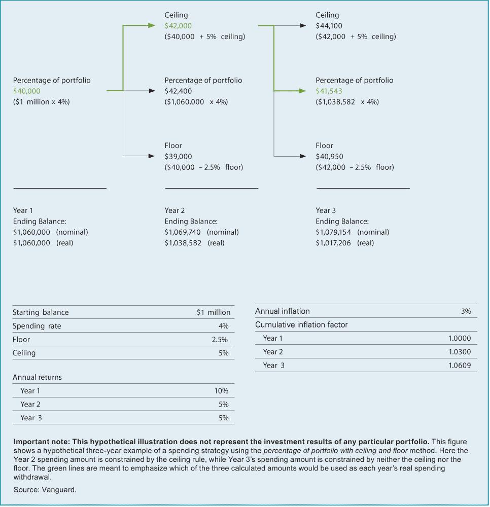
As in the percentage of portfolio strategy, the investor calculates each year’s spending by taking a stated percentage of the prior year-end portfolio balance. The investor then also calculates a ceiling and a floor by applying chosen percentages to the prior year’s spending amount (our scenarios used a 5% ceiling and a 2.5% floor—see Appendix 2 for an illustration). The investor then compares the three results. If the newly calculated spending amount exceeds the ceiling, the investor limits spending to the ceiling amount; if the calculated spending is below the floor, the investor increases spending to the floor amount.
Although with this method spending will vary from year to year based on what the markets do, it is not allowed to exceed a set range as long as assets remain in the portfolio—a factor that can assist with short-term planning. The strategy allows investors to benefit from good markets by increasing spending, while in less favorable periods it prompts investors to reduce spending, thereby supporting the portfolio’s longevity. By periodically monitoring the portfolio and allowing for some flexibility in annual spending based on recent market performance, investors can improve their likelihood of meeting long-term financial goals.
Table 4. Summary Statistics for Three Variations of Ceiling/Floor Strategy
|
Portfolio Strategy
|
Variation 1 | Variation 2 | Variation 3 |
|
Ceiling
|
0.0%
|
5.0%
|
10.0%
|
|
Floor
|
0.0%
|
2.5%
|
10.0%
|
|
Portfolio survival rate
|
78%
|
92%
|
100%
|
|
Real (inflation-adjusted) ending asset balances
|
|||
|
Maximum
|
$100,030,300
|
$88,954,400
|
$73,136,800
|
|
75th
|
$3,162,400
|
$2,220,400
|
$2,174,500
|
|
Median
|
$1,153,700
|
$1,068,600
|
$1,194,400
|
|
25th
|
$102,400
|
$449,700
|
$659,000
|
|
Minimum
|
$0
|
$0
|
$6,500
|
|
Real annual spending as a percentage of initial spending
|
|||
|
Maximum
|
100%
|
525%
|
2555%
|
|
75th
|
100%
|
198%
|
209%
|
|
Median
|
100%
|
114%
|
117%
|
|
25th
|
100%
|
66%
|
67%
|
|
Minimum
|
0%
|
0%
|
3%
|
|
Percentage of time real spending drops below initial spending
|
6%
|
45%
|
47%
|
|
Important note: This hypothetical illustration does not represent the investment results of any particular portfolio.
|
|||
|
See the box above for guidelines on withdrawal rates in this analysis and Appendix 1 for details on the VCMM simulation, including return assumptions.
|
|||
|
Source: Vanguard.
|
|||
When it comes to real annual spending amounts, we found that applying the ceiling and floor constrained both the upside and the downside. In our simulation, the highest annual spending level reached with this strategy was 525% of the original target; by contrast, the percentage of portfolio strategy reached a maximum of 3,634%. On the other hand, the ceiling/floor limits produced fewer scenarios in which annual spending fell below the target level: 45%, compared with 48% for the percentage of portfolio strategy. These differences reflect the moderation imposed by the ceiling and floor.
Compared with the dollar amount grown by inflation strategy, the ceiling/floor method had a higher maximum-spending scenario (525% of the original target versus 100%), but it also had many more cases in which spending dropped below that target (45% versus 6%). This is because, under the dollar amount grown by inflation strategy, inflation-adjusted spending is kept at a constant level, instead of being allowed to rise to a ceiling or held up above a floor.
The most important consideration for the percentage of portfolio with ceiling and floor strategy is the selection of the upper and lower percentages that will be applied to the prior year’s spending. The narrower the spread between them, the more similar this strategy is to the dollar amount grown by inflation strategy, and the more likely that the portfolio could reach a crisis point at some future time. The wider the difference between the ceiling and floor percentages, the more similar this strategy is to the percentage of portfolio strategy. That is because calculated spending reaches the ceiling or floor relatively rarely, leaving the withdrawal percentage as the primary factor in annual spending fluctuations.
To demonstrate this point, we repeated the ceiling/floor simulation analysis with two variations: a 0% ceiling and floor, and a 10% ceiling and floor. As shown in Table 4, the results for those variations are quite similar to the results for the two other strategies (shown in Table 2). This is because the 0% variation—in which inflation-adjusted spending has no room to fluctuate—is essentially the same as the dollar amount grown by inflation strategy, and the 10% variation, with its hard-to-reach limits, is quite similar to the percentage of portfolio strategy. The outcomes for other ceiling/floor combinations between 0% and 10% would likely fall between these values.
Although we believe that investors can usefully analyze these conceptual spending frameworks, we also recognize that most investors determine their annual spending in a less rigid way. Certainly no strategy should be followed blindly; indeed, it is essential for investors to periodically evaluate their income strategies, assess their portfolios, and consider whether alterations are needed.
Still, working through calculations such as these on an annual basis can assist investors with their long-term planning as they strive to achieve their financial goals. In our view, flexibility is the one word that best describes a prudent spending strategy. Rigid spending rules cannot eliminate investment volatility; they simply push its consequences into the future. Spending strategies insensitive to returns are risky, in that they assume a portfolio will recover before a crisis point is reached—at which time much more dramatic reductions in spending would be necessary.
If a portfolio is to rely on the capital markets for growth, investors must either accept continuous, relatively smaller changes in spending or else risk having to make abrupt and significantly larger adjustments later. The more investors can tolerate some short-term fluctuations in spending, the more likely they are to achieve their longer-term goals.
Keep in mind, however, that although this strategy provides for some reduction in spending in poor markets, it does not preclude the possibility of a substantial decline in the portfolio’s principal, which could require spending to drop below the “floor” and could even result in premature portfolio depletion. In our simulation, 92% of the paths resulted in a positive ending portfolio balance after 35 years. As expected, this 92% value lay between the survival rates for the other two approaches (78% and 100%).
Financial Planning
Financial Planning

Herb Schrayshuen from NY posted over 12 years ago:
David Dudley from CT posted over 12 years ago:
John Morgensen from NV posted over 12 years ago:
Norm from Massachusetts posted over 12 years ago:
Nathan Busch from MN posted over 12 years ago:
George Pitonyak from NC posted over 12 years ago:
Keith Shadrick from IN posted over 12 years ago:
H Kinsling from CA posted over 12 years ago:
Mike from OH posted over 11 years ago:
You need to log in as a registered AAII user before commenting.
Log InCreate an account