


Raymond Rondeau leads a class in AAII's new Essential Investing Video Course. Go to https://www.aaii.com/ves for more information and to subscribe.
This second part of our series on the relative strength index (RSI) is for the more advanced or inquisitive investor who wants to understand in greater depth some of the intricacies of RSI and its calculations. I discuss how calculating RSI has changed over time, some of the indicator’s oddities and why its values can differ slightly from platform to platform. Additionally, I cover a few of the “customized” variations of RSI, which attempt to contour or compensate for certain attributes.
For part one of the series, “Classic Technical Indicators: The Basics of the RSI,” click here.
Before progressing, it is critical to note that the calculations in the following tables and their respective values are theoretical and that they have been contoured for illustrative purposes only. Furthermore, the associated calculations and their output values have been modified in various manners and as appropriate to each section for the sole purpose of illustrating each covered concept.
RSI vs RS
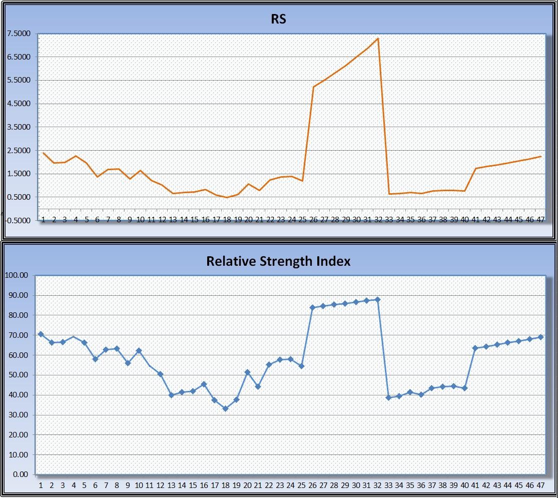
The shape of the RS from RSI’s formula (not relative strength) and the final RSI value are similar but with a varying amplitude. The “RSI” portion of the formula simply “compresses” or calibrates the RS value into an oscillating range for easy identification of stretched levels. “Stretched” levels is not the same as overvalued. In this case, “stretched” is referring to the opposite of compression of the RSI formula to the 0–100 range. Without this compression, the values would be extreme and incomparable from issue to issue as they would be “stretched” to all kinds of readings. Also, there could be no overbought or oversold readings without compression.
Note: The referred to “RS” in Wilder’s RSI formula and this article (unless noted), is not the same as the traditional definition and measurement of “relative strength.” I have differentiated the two by replicating the “RS” designation used in Wilder’s formula as “RS” and calling the more popular calculation “relative strength.” More about the distinction between the two was covered in part one of this series, and even more specifics will be covered in part three.
In review from Part I
Wilder’s original RSI calculation formula.
RSI = 100 – (100 / (1 + RS)) or 100 * (RS / (1+RS))
RS = Average Gains (over the period) / |Average Losses| (over the period)
Wilder’s Smoothing Average
Average Gains over the Period (smoothed) = (((Average Gains MA) * (n – 1)) + Current Bars Gain ) / n
Average Losses over the Period (smoothed) |Absolute value| = (((Average Losses MA) * (n – 1)) + Current Bars Loss ) / n
Wilder’s Smoothing Average (WSA)
Deeper examination of Wilder’s Smoothing Average (WSA) shows that it is similar to an exponential moving average with many of the same advantages.
- WSA responds quicker to price changes by giving more weight to recent price movements.
- WSA incorporates all the historical data being referenced as opposed to having abrupt changes that can cause distortions.
For example, with a 200-period simple moving average (SMA), the price of a bar 200 periods ago would have the same influence as the price action of just one bar ago. If we accept that the most recent price action should be more relevant to our current analysis, then this would not be the most efficient approach. Similarly, with this SMA example, the price action of 201 bars ago would not have any relevancy at all and the price action of a bar 200 periods ago would be included. Here we would be creating a purely arbitrary quantitate barrier, which would also not be logical or efficient. Both of these concerns are addressed by both exponential moving averages (EMAs) and WSA.
In reality, Wilder’s Smoothed Average is actually just a smoothed exponential moving average (EMA), with its results paralleling an adjusted slowed exponential moving average. The conversion formula is:
EMA = (2 * WSA) – 1 or WSA = (EMA + 1) ÷ 2
14 period WSA = 27 period EMA | 20 period WSA = 39 period EMA
Furthermore, some technicians will calculate the RS average gains and average losses with other MAs. For instance, some will attempt to use a straight simple or exponential moving average as opposed to the traditional Wilder’s Smoothed Average.
When RSI Isn’t RSI
Because of the timing of the release of RSI in 1978 and the subsequent development and utilization of computers and the increased amounts of data available, variations of calculating the RS in RSI have evolved.
RSI’s Positive Calculation Bias
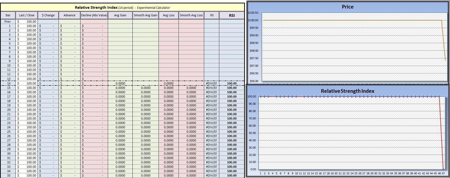
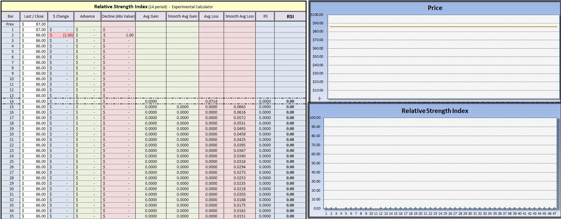
Delving into the numbers of RSI points out an interesting anomaly with Wilder’s original calculation method. As mentioned in the beginning of part one, when there are no losses, RSI will set its value to 100. But the same value would persist if there are no price gains either, as we can see in the table below. Because of this relationship, one could theorize that RSI can have a “positive calculation bias” in this situation.
With no pricing changes at all, we would expect the RSI value to be at a level of 50 as opposed to 100. This can be misleading to the RSI user who “correctly” associates a value of 100 with positive pricing strength and who is unaware of this phenomenon.
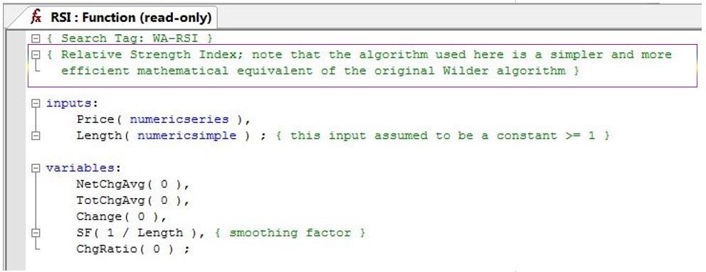
Fortunately, most technicians, platforms and formulas now compensate for this effect with alternate calculation methods, so the value is set to 50 when prices meet this situation. Remember, by calculation (gains to losses) RSI values above 50 are considered bullish and RSI values below 50 are considered bearish. Therefore, the accepted belief is that when there is no price change, RSI is neutral and the value should be 50. This is why most technical analysis platforms adjust for these situations.
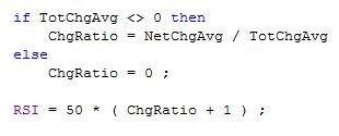
Here we see TradeStation’s EasyLanguage code showing how an RSI “else” situation of: no changes or a zero value, calculates and plots an RSI value of 50.
Change Ratio = 0
RSI = 50 * (0 + 1) = 50
RSI’s Persistent Memory Dilemma
The majority of technicians calculate RSI using WSA, and rightly so, due to some of the advantages that just covered. But because WSA weights recent price changes and incorporates all the data loaded into a chart there are a few rare (really hypothetical) mathematical situations where RSI could give a user a false impression. This can occur when RSI has been printing an extreme bullish or bearish reading when there haven’t been any price changes for an extended period of time.
RSI’s Price Weighting Bias
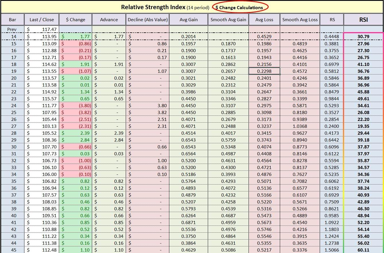
Because Wilder’s RS values are calculating off of actual dollar changes as opposed to percentage changes, this can create a small price-level bias in an issue that has experienced a dramatic price level change, over the “N” periods RSI is referencing.
This phenomenon occurs with using dollar amount change calculations, because price changes occurring at lower numbers, are NOT being given a different “percentage relevancy” as price changes at higher price levels. This is similar to the effect that we see with calculations of the “price-weighted” Dow Jones index, where higher-priced stocks have a greater influence on the reported index’s performance. This well-known distortion also occurs with the utilization of arithmetic scaling (as opposed to semi-logarithmic) on price charts.
Stock ABC goes from $10 to $30 in two days:
Price goes from $10 to $20 RS = + 10 100% increase
Price goes from $20 to $30 RS = + 10 50% increase
For example: In the table above, we see that a price movement from $10 to $20 results in a 100% increase in price but the same $10 price movement, from $20 to $30 results in only a 50% increase. Projecting this to the RS calculation in RSI, we can see how this can be somewhat misleading, in certain situations. This occurs because the RS is calculating off of the actual dollar change, and therefore it would give the $10 gain the same relevancy at both price levels, even though one was a 50% gain and the other a more substantial 100% gain.
In truth, even price movements on highly volatile stocks or on most issues’ weekly charts only vary moderately, but because this deviance is repeated after every bar, theoretically it is worth noting. Regardless of the method of calculating the RS portion of RSI, either with straight dollar changes or percentage changes, RSI’s shape and values will remain relatively close.

RSI—The Inverse Dividend Relationship
In this study, we can see how a company’s potential improving strength can actually work inversely and hurt or lower RSI’s values. This phenomenon can occur because the RSI formula is based off of the closing price of the issue, creating a scenario where a company paying a higher dividend, becomes penalized by RSI and its calculation method. This happens because the dividend is not factored in as part of the return or included in RSI “strength” calculations and readings.
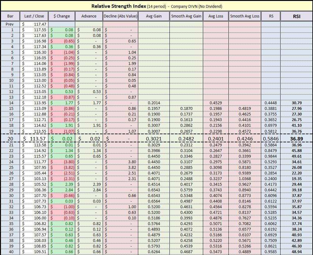
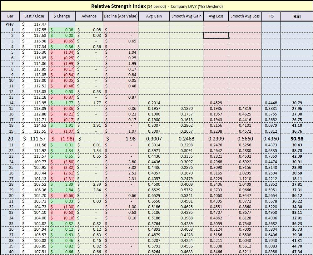
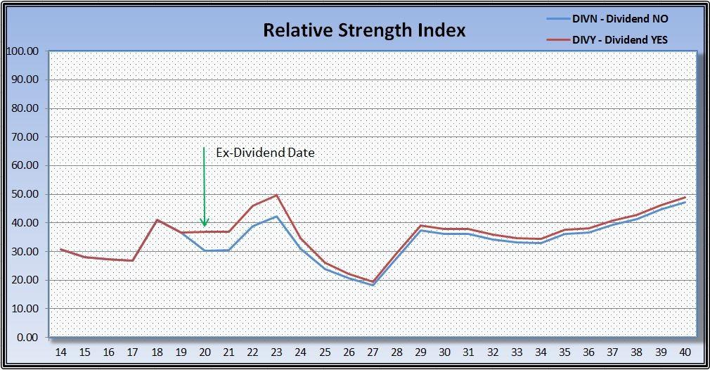
In this example, we assume that we have two hypothetically identical companies all with the same fundamentals: DIVY (Dividend Yes) and DIVN (Dividend No). We also assume that DIVN pays no dividends but on day 20 DIVY’s (ex-dividend date), there is a $2.00 dividend per share. In this scenario, company DIVN’s stock price would obviously remain the same at $113.57 (as it did not pay a dividend) and it has a subsequent RSI value of 36.89. In the DIVY example, the price of its stock drops by the approximate amount of the dividend paid, to $111.57. Relative strength aside, this is what happens when a company trades ex-dividend; its stock price is lowered by the amount of the dividend payment. This happens very quickly on a company’s ex-dividend date and most investors don’t realize the price decline. Because of this necessary change in price, its RSI value NOW falls over 17%, to a value of 30.36. Again, further inspection of the tables also confirms, as we would expect, that all subsequent RSI values would also be systematically lowered.
For dividend-paying companies, we can clearly see that the subsequent approximate drop in price (to offset the dividend payment amount on the ex-dividend date) negatively affects the stock’s RSI numbers. This creates an interesting, but often unknown, inverse relationship; where a higher dividend payment, on presumably a stronger company paying that amount (not true in all situations but generally higher dividend distributions over time are associated with stronger, more mature firms), would more negatively affect its RSI’s readings.
Explanation of Dividends & Price Activity
Although often disputed, the relationship between the approximate drop in the market price of a stock to offset the dividend payment amount on the ex-dividend date theoretically has to exist. If it did not exist, then investors would simply purchase a stock the day before it goes ex-dividend and then sell it immediately after (some investors still try this) in an attempt to capture the dividend.
As we know there are “no free rides on Wall Street” and you can’t get a net quarterly, semiannual or annual dividend payment gain for holding a stock for a day or less for nothing. The inevitable offsetting drop in the stock price is the neutralizer to this shortcut “dividend capture” approach that attempts at getting something (dividend) for nothing.
RSI—Stock Splits & Reverse Splits
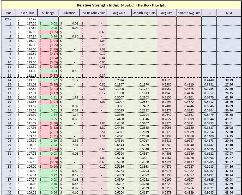
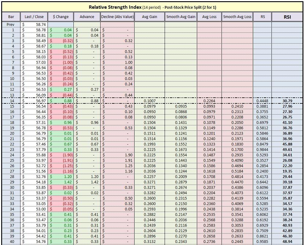
Interestingly with split activity, because the proportion of the related price change to the base price doesn’t change, the associated RSI values also do not change. This is similar to observations from both the market and individual investor’s perspective when analyzing split activity.
For example, in a standard 2-for-1 split:
From a broad market perspective, the number of outstanding shares will change (double in our example) but the price will drop by the same ratio, leaving an equal pre-split and post-split market capitalization.
Pre-Split: 1,000,000 shares at $200 / share = $200 Million Market Cap
Post-Split: 2,000,000 shares at $100 / share = $200 Million Market Cap
From an individual investor’s perspective, their number of held shares will also adjust (double in our example), but the price will again drop by the same ratio, leaving them with the same pre-split and post-split total position value.
Pre-Split 100 shares at $200 / share = $20,000 Total Position Value
Post-Split 200 share at $100 / share = $20,000 Total Position Value
In relationship to RSI, because its algorithm derives its values from the charted values and because the vast majority of charted values are all back adjusted to reflect past split activity, there is essentially no change in its final readings. This is one reason that for most circumstances, it is preferred to use the standard adjusted price history, on most platforms and charts, for the majority of technical studies. A hypothetical RSI example confirming this stock split relationship is shown below.Note: Standard practice is to adjust for split activity but not dividends.
RSI Data Length Dependency
Another oddity of calculating RSI is that the ending value will be dependent on how far back the data is initially referencing for its first calculation. This is due to the fact that although the RS average gains and losses incorporate a smoothing average technique, the first “average gain” and “average loss” is determined by how much data is being referenced by the chart. The further back one references the data, the less likely this effect will be and the more accurate RSI values should be. As a general rule, for daily charts many technicians consider loading at least 252 bars of data (the number of trading days in a year).
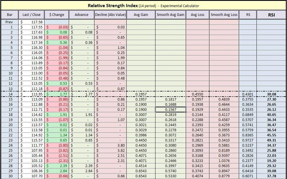
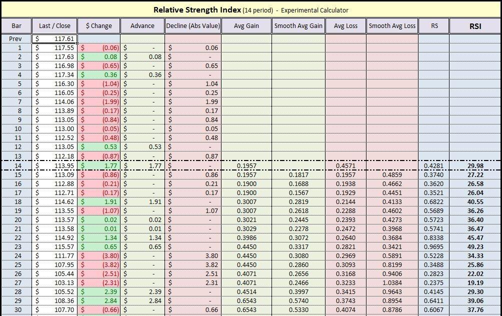
If one were using RSI crosses up from the oversold RSI level of 30 for their execution signals, we can see that in this example, the amount of data referenced in the chart could have altered a potential future signal. Further examination of later calculated bars (15–30), shows that RSI’s values predictably continue to differ, despite the fact that each new bar’s price is exactly the same.
In reality, the smoothed values that are dependent on when you start calculating the average, would likely not be this dispersed. Nevertheless, this example does reinforce the influence that the amount of data loaded into a chart can have on RSI’s value. This addresses a common question of why RSI’s values can differ from platform to platform, even when utilizing the exact same algorithms.
RSI—Mending the Methodology
Cutler’s RSI
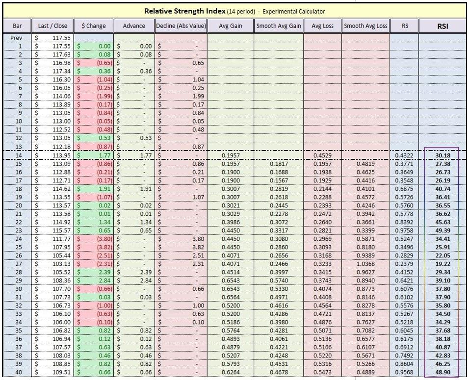
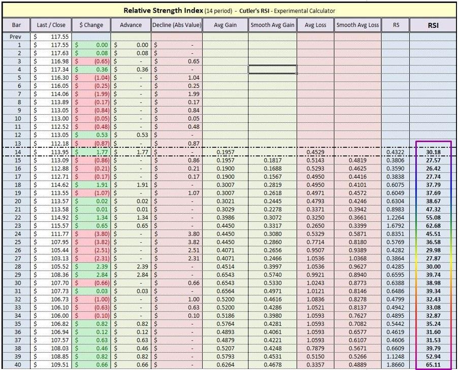
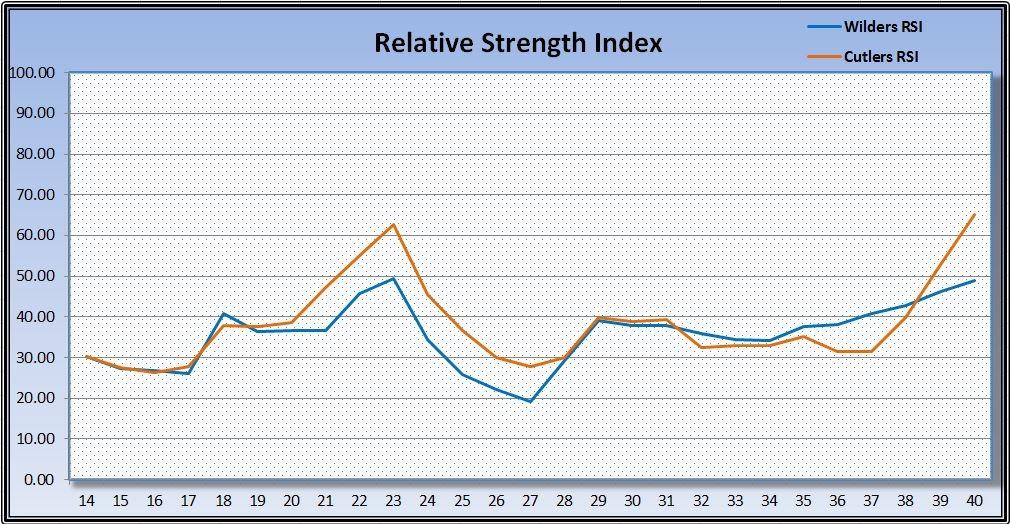
As mentioned earlier, one method of neutralizing some of these factors, including this data referencing effect is by using a simple moving average (SMA) as opposed to WSA. There is a variation of RSI called Cutler’s RSI that eliminates this “data length discrepancy” as he referred to it. Of course, although it does eliminate the data length issue, it does so at the expense of abrupt price cutoffs and losing the “believed” advantage of weighting the most recent price action. With Cutler’s RSI the RS is calculated as:
RS = SMA (gains over n periods) ÷ |SMA (losses of n periods) |
Alternate Refinements
Even after acknowledging these RSI price-event relationships, the majority of RSI users will still apply the base RSI indicator on standard normalized data and charts. For the more advanced user and in specific situations, one could consider using specialized adjusted price data (dividends and other corporate actions) to minimize some of these covered RSI event distortions. For example, by using adjusted data on extremely high dividend paying stocks, this approach would theoretically “purify” and smooth RSI’s values.
Some investing platforms do provide this as a charting option. One pure data source that provides this, free of charge for download, is Yahoo’s “Adjusted Close.” This data adjusts the closing prices for previous and current corporate actions and distributions.
More information can be found at Yahoo’s help page here.
Another approach that an investor may want to consider incorporating is to consistently use the same platform and sets of RSI indicators. If one does this and references a large amount of data (diminishing the “data discrepancy effect”) this can keep the readings and interpretations consistent and relative.
Lastly, more experienced investors may want to consider utilizing variations of the original RSI formula itself to further compensate for these factors covered throughout this section. In fact, this is something that will be covered in Part IV of this series, including backtesting comparisons of a modified RSI version to the original formula covered here in detail.
Conclusion
Although potentially beneficial, I think most technicians would agree, it is not necessary to completely understand all of the mathematics and intricacies of RSI calculations to effectively use this indicator.
The key points to be aware of from this article are:
- That RSI’s values are not perfect. RSI calculations and methodology have changed over time and they should be analyzed and questioned.
- RSI calculation methods could vary from site to site and platform to platform and there are mathematical reasons for this.
- Acknowledging that variance in RSI values exist, can help investors keep RSI’s readings in perspective, reinforcing that they are not necessarily an exact science or prophetic in nature.
Discussion
FREE REPORT

Scott Juds from WA posted over 8 years ago:
You need to log in as a registered AAII user before commenting.
Log InCreate an account