

Related

Technical Analysis
The market’s best and worst months have been clustered together. A trend-following strategy can help investors avoid extreme volatility.
by Adam Butler | October 2017
The asset management industry is fond of reminding investors how much money they leave on the table when they miss the 10 best monthly returns.
What they fail to mention is that, because stock market volatility clusters during periods of market crises, the best monthly stock market returns are directly adjacent in time to the worst monthly returns.
Consider the following examples: The worst months of 2001 and 2009 occurred in February and, coincidentally, the best months occurred in April of the same years. Similarly, the worst months of 2002 and 2011 both occurred in September and the best months in October of those years. These are just a few examples of many where this clustering occurs.
Investors could bypass the large price fluctuations by missing both the best and worst days or months in the market. These investors would realize similar returns as buy-and-hold investors, but with much less grief in the form of volatility and drawdowns.
This article examines the experience of investors who miss the 10, 20 and 50 months with the most extreme returns in either direction. You will see that investors who sidestep these months harvest similar returns, but with a much smoother ride. A simple, time-tested method to sidestep these months is described. The method is then tested on a variety of other markets with similar success. Finally the concepts are tied together into a diversified strategy.
In terms of long-term total returns, missing the best months is roughly equivalent to missing the worst months, just in the opposite direction. For example, since 1900, investors would have realized approximately 2% per year lower returns if they’d missed the best 10 months, but they would have added about 2% per year from missing the 10 worst months. In fact, you can see from Figure 1 that investors who miss both the 10 best and worst months end up with slightly better returns than the market, but with much less volatility and smaller drawdowns.

In fact, there is a progressive improvement in returns, with commensurate reductions in both volatility and maximum drawdowns, as increasing numbers of best and worst months are excluded. An investor who managed to miss the 50 most-extreme monthly returns would have experienced slightly higher compound returns (9.9% annualized) than a buy-and-hold investor (9.6% annualized), with 25% less volatility (13.2% versus 17.6%) and less than half the maximum drawdown (45.35% versus 83.66%).
Volatility is defined here as the annualized daily standard deviation, meaning the variance around the daily average return. Maximum drawdown is defined as the largest percentage peak-to-trough loss. Despite missing 50 monthly returns, this investor would have been in the market almost 97% of the time.
If we can improve risk-adjusted performance by avoiding the best and worst months, and these months tend to cluster together during periods of market crisis, it prompts the question: Is there a simple way to avoid these extreme periods? It turns out there is. Simple trend-following/momentum rules are effective for exactly this reason. They work because extreme returns tend to occur when markets are in steep downtrends.
Consider a simple strategy that holds the S&P 500 index for the following month if the index is above its 10-month total return moving average on a monthly close. Cash is held instead if the S&P 500 is below its 10-month moving average.
For those unfamiliar with moving averages, they are a simple way of smoothing noisy data such as stock prices, making it easier to judge the direction of an underlying trend. For this article, the average of monthly total returns over rolling 10-month periods is used. The 10-month moving average is consistent with the more ubiquitous 200-day moving average, except that price relative to the average is observed only at the end of the month.
The advantage of observing the trend less regularly is that the strategy is less vulnerable to intra-month noisy whipsaws. On the other hand, monthly observations may fail to catch major intra-month turning points, and capture slightly more downside. This is analogous to the “signal-to-noise” ratio from engineering and information theory and is a common trade-off in markets.
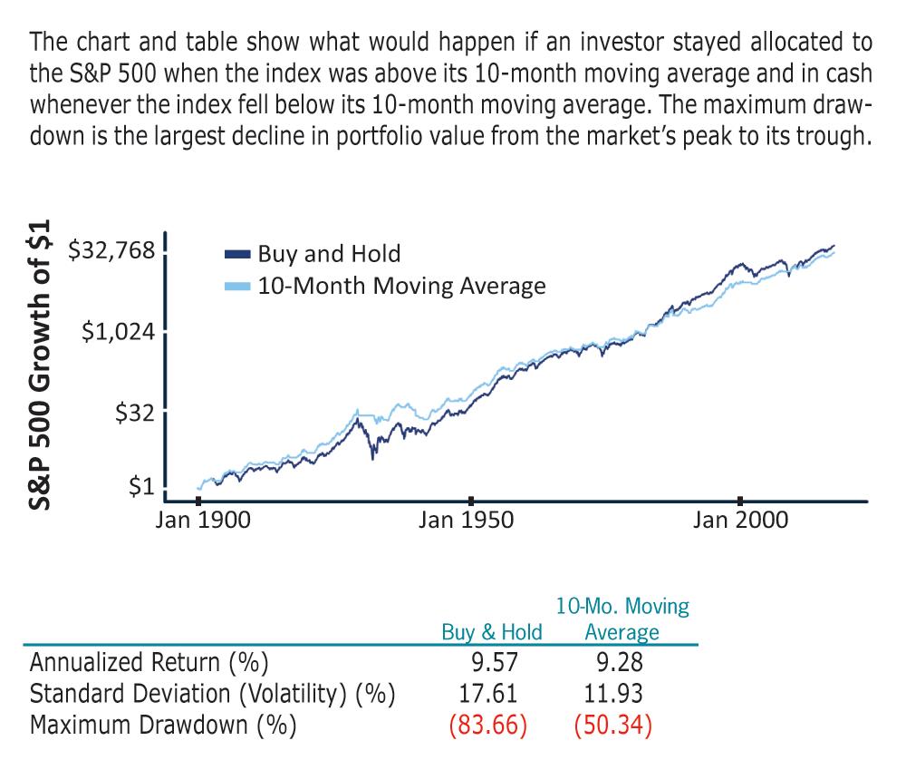
From a risk-adjusted performance perspective, a simple 10-month moving average rule—a simple indicator of positive or negative momentum—produced results that are competitive with what is observed from a strategy that manages to avoid the 50 best and worst months since 1900, as shown in Figure 2. The 10-month moving average strategy realized an annualized return of 9.28% with a maximum drawdown of 50.34%. Of course, these results aren’t quite as good as simply avoiding the best and worst months, since the 10-month moving average does not have perfect foresight. (The results for the 10-month moving average strategy assume the investor earns 0% returns when not invested in the market. Performance of the tactical strategy would improve if the investor earned interest on the cash position.)
Were this phenomenon isolated to U.S. stocks, it might be easy to dismiss. But very similar performance is observed from a variety of asset classes above and below their respective 10-month moving averages. Specifically, most asset classes yield significantly higher returns, with lower volatility, when they are in a positive trend.
When evaluating the strategy using U.S. stocks, foreign stocks, U.S. Treasuries, real estate investment trusts (REITs) and commodities, the state of the price series is observed relative to the moving average at the end of each month, and the appropriate investment posture is applied to returns in the following month. (Note: While many studies use monthly total return data, daily total return data is used to illustrate ranges of outcomes that could not be well explored at a monthly frequency.)
Quite a substantial improvement in risk-adjusted performance is observed when the five assets above are combined into a global tactical asset allocation (GTAA) strategy. Specifically, each of the aforementioned assets is held in equal weights—20% of investment capital in each asset—when they are above their 10-month moving average. When an asset moves below its moving average, that asset’s weight (20%) is held in cash the next month. This strategy benefits from a combination of robust diversification, and a history of avoiding the most volatile months in each asset class. Note that this simple strategy—first described by Mebane Faber in his 2006 working paper, “A Quantitative Approach to Tactical Asset Allocation”—produced returns competitive with those of a traditional 60% stock/40% bond portfolio (8.3% versus 8.9%), but with less volatility and less than half the maximum drawdown from November 1992 through August 2017 (15.5% versus 32.3%).
Importantly, the GTAA strategy is a simple, rules-based strategy that does not rely on gut instinct, macroeconomic analysis, narratives, political insight or any other discretionary intuition. It is a systematic approach that is based on time-series momentum. It may not be the best way to harness this effect, but it is remarkably effective for such a simple strategy.
Of course, active strategies require discipline, time and effort. It’s easy to show a simulation that has made every trade, flawlessly executed, without the interference of human emotion or distraction. However, since a human must ultimately hit the buy or sell button at each rebalance period, we cannot discount our trepidation when situations or environments are less than ideal for making a trade. We also get sick, take vacations, lose power or get stuck in other human situations that make it difficult to follow each trade signal in a timely manner. This prompts the question: What if we were a week or two late to take a trade? What about a month? After all, any change in the timing of these trades will definitely alter the outcome.
Consider the emotions of an investor following the GTAA approach when they were told to move entirely out of equities in September 2000, after years of a massive bull run. On that date, the S&P 500 was a modest 5.5% off of its March 2000 peak. Or how about the pause an investor may have felt when they observed a signal to re-enter equities in June 2009, with a nation still reeling from the worst economic downturn in a generation? Even though the equity market was nearly 40% above its March 2009 bottom, an investor’s appetite for risk would have been understandably shaky.
As demonstrated in Table 1, delaying or missing occasional trades will likely not have a disastrous effect on returns, leaving the majority of the benefit intact. Even investors who delay taking trade signals for up to three weeks haven’t faced a material decay in performance historically. This is a promising test of robustness for this simple strategy.
Table 1. The Impact of Delaying to Follow a Trading Signal
| Postponing to follow through a trading signal by up to four weeks reduces returns, but not significantly. The results in the table show the returns for a five-asset diversified portfolio following the global tactical asset allocation (GTAA) strategy. | |||||
| GTAA Strategy | |||||
|---|---|---|---|---|---|
| 0- Week Delay | 1- Week Delay | 2- Week Delay | 3- Week Delay | 4- Week Delay | |
| Annualized Return (%) | 8.26 | 8.57 | 8.1 | 8.37 | 7.83 |
| Standard Deviation (Volatility) (%) | 7.29 | 7.22 | 7.17 | 7.23 | 7.42 |
| Maximum Drawdown (%) | -15.52 | -13.53 | -13.53 | -13.53 | -14.07 |
| Source: ReSolve Asset Management. Data from CSI data and underlying index providers where data for investable funds have been extended prior to their date of inception. The results are hypothetical results and are NOT an indicator of future results and do NOT represent returns that any investor actually attained. | |||||
One might also envision a situation where an investor fails to take a trade signal altogether. As previously mentioned, shell-shocked investors in June 2009 may have recoiled against the suggestion they should redeploy their savings back into equities. Worse, each subsequent month of gains may have made it increasingly difficult to invest. There were many investors who, having failed to take the buy signal in 2009, remained out of the market until the first major correction in 2011.
Given how easy it is to imagine this scenario, the impact of completely missing a full trade signal was analyzed. Specifically, the distribution of results for investors who missed just one full rebalance signal was analyzed. There are about 50 complete buy-sell cycles per asset in the testing from 1991, for a total of about 250 complete missed trades. Table 2 illustrates and quantifies the results of these tests at the 0th, 5th, 25th, 50th, 75th, 95th and 100th percentiles. The 0th percentile result is the worst result of the 7,000 tests, with an annualized return of 6.2%. The 100th percentile represents the best result, with an 8.4% annualized return. Results were better than the 5th percentile (7.2% annualized return) 95% of the time, and better than the 95th percentile (8.2% annualized return) just 5% of the time. The 50th percentile is the median result with a 7.8% annualized return. To put these numbers into perspective, a buy-and-hold strategy that was rebalanced monthly realized an annualized return of 6.7%. Clearly missing a trade can reduce returns, but the impact is rarely catastrophic.
Table 2. The Impact of Missing a Full Rebalance Signal
| The table below shows how missing one full buy-sell signal impacts the returns in a five-asset, diversified portfolio following the global tactical asset allocation (GTAA) strategy. The 0th percentile represents the worst result, while the 100th percentile represents the best result. | |||||||
| Percentile | |||||||
|---|---|---|---|---|---|---|---|
| 0th | 5th | 25th | 50th | 75th | 95th | 100th | |
| Annualized Return (%) | 6.17 | 7.22 | 7.62 | 7.85 | 8.03 | 8.19 | 8.44 |
| Standard Deviation (Volatility) (%) | 5.75 | 6.45 | 6.74 | 6.87 | 6.97 | 7.16 | 8.45 |
| Maximum Drawdown (%) | -29.95 | -17.74 | -15.52 | -15.52 | -14.86 | -12.78 | -9.69 |
| Source: ReSolve Asset Management. Data from CSI data and underlying index providers where data for investable funds have been extended prior to their date of inception. The results are hypothetical results and are NOT an indicator of future results and do NOT represent returns that any investor actually attained. | |||||||
The simple moving average system described in this article produces an average of four round-trip trades per asset class (with each asset class represented by a single exchange-traded fund) per year. Some investors may be concerned about the impact of taxes and costs for a strategy with this level of trading.
To estimate the costs of implementing the strategy for a typical private investor, $5 per trade is assumed, as this is a popular price point for large online brokerages. Multiplying $5 per trade times four trades per ETF by five ETFs amounts to about $100 per year in trading costs ($5 x 4 x 5 = $100), or 0.1% of a $100,000 portfolio—roughly in line with the expense ratios of the least-expensive ETFs. (The trading cost excludes the expense ratio charged by each ETF, a cost that would also be incurred by a buy-and-hold strategy.)
Given that the strategy turns over the portfolio on average at least once per year, it’s reasonable for investors to be concerned that many trades will be taxed at the much higher short-term capital gains rates. There are some nuances around this, as trend-following strategies tend to generate a large number of small short-term losses with a few large long-term gains. This said, let’s assume the losses, gains and timing of trades are equally distributed through time. An investor might be tempted to hold off crystallizing gains on a trade until they had held the ETF representing the specific asset class for at least 12 months, in order to qualify for more advantageous long-term tax treatment.
The results for an investor who tries to manage this tax risk can be investigated. Consider a slight alteration to the five assets in the global tactical asset allocation strategy previously discussed. What if, when presented with a buy signal, an asset was held for a minimum of 13 months before taking the next sell signal as a way to minimize short-term capital gains?
Doing so materially impairs the performance of the strategy. Returns drop by about 1% to 7.29% over the period of 1991 through August 2017 (versus 8.26% for the standard GTAA strategy.) Volatility rises, and the maximum drawdown increases from 15.5% to 24.6%. This illustrates an important lesson for investors wishing to employ an active approach to their portfolios: We can have the full risk management potential of our systematic strategy with taxes or no risk management without. There is no free lunch.
Moving averages provide a simple, time-tested method to avoid the most volatile, least productive months in markets. These tools work even better in conjunction with thoughtful diversification.
A 10-month moving average strategy applied in equal weight to a group of five diversified asset classes has produced very attractive returns with less risk and smaller losses than more traditional balanced portfolios of stocks and bonds.
Technical Analysis
Trading Strategies


Mark Pankin from VA posted over 8 years ago:
James Vanek from AZ posted over 8 years ago:
John Young from MA posted over 8 years ago:
Peter Urso from IL posted over 8 years ago:
Steve from CA posted over 8 years ago:
Bhaskar Bhattacharya from BC posted over 8 years ago:
William Anderson from IL posted over 8 years ago:
William Gibson from MO posted over 8 years ago:
You need to log in as a registered AAII user before commenting.
Log InCreate an account