Google offers several productivity apps that allow users to create documents, spreadsheets and presentations and access them from any computer, anywhere in the world, for free. These apps are called Google Docs, Sheets and Slides. In this Spreadsheet Corner, we concentrate on Google Sheets. Google Sheets is an online spreadsheet app that lets you create and format spreadsheets and simultaneously work with other people.

Introduction to Google Sheets

Google lists these features in their Google Sheets explanation:

• Import and convert Excel, .csv, .txt and .ods formatted data to a Google spreadsheet
• Export Excel, .csv, .txt and .ods formatted data, as well as PDF and HTML files
• Use formula editing to perform calculations on your data, and use formatting make it look the way you’d like
• Chat in real time with others who are editing your spreadsheet
• Create charts with your data
• Embed a spreadsheet, or individual sheets of your spreadsheet, on your blog or website

Google Sheets works similar to Microsoft Excel in that you can enter formulas into the spreadsheet and perform functions accordingly. You can also pull data directly from Google Finance using the GOOGLEFINANCE function. Google Sheets offers such functions as spell check, insert charts, print, share online and insert formulas. While Sheets only offers a small portion of the capabilities that Microsoft Excel has, it is a viable alternative to Excel since the basic functions are all that most spreadsheet users would need. Would it work for individuals who use Excel to its fullest potential? Most likely not.

One useful feature is that sheets are automatically saved as you work, so you do not have to click save all the time. Also, Google Sheets lets users access their spreadsheets offline, even without Internet access (only available through the Google Chrome browser). Simply by clicking “enable offline editing,” users can work in their browser or pin files to their mobile device. Entering formulas is similar to Excel; users type in an equal sign and an open parenthesis followed by a formula and a closed parenthesis. Sheets recently added an autocomplete function, which offers suggestions as you type. Users can minimize or maximize the help box by clicking F1. Also similar to Excel, Google Sheets supports several tabs in one sheet and tabs can be linked to one another. Google Sheets offers several different add-ons as well as apps for iPad, Android and iPhone. It is possible to add array formulas or import data from various structured data types, including XML, HTML, CSV, TSV, RSS and ATOM XML feeds. Users can also perform queries written in the Google Visualization API Query Language.

I found that when I tried to open a Google Sheets document created on my PC on my iPad, I couldn’t open it easily. It was at that time that I realized you need to download the Google Sheets iPad app in order to use it correctly, but it still didn’t open with the exact same formatting. As I mentioned before, Google Sheets doesn’t have all the formulas that Microsoft Excel contains but there are several formulas that overlap. I think that Google Sheets is a viable free alternative for those attempting basic Excel-related functions, and improvements continue to be made to the program.

We used Google Sheets to create a rudimentary portfolio tracker. This is a simple portfolio tracking spreadsheet that allows users to input current equity holdings and keep track of their current values and track securities through a watchlist.

The Spreadsheet

CI’s Portfolio Tracker with Google Sheets contains two different tabs: Portfolio and Watchlist. Cells highlighted in yellow require manual input, while everything else will be calculated accordingly. CI’s Portfolio Tracker with Google Sheets will appear once you click this link.

In order to have your own copy that you can edit you have several options. The first one requires you to sign in to Google, then click File, and Make a Copy. You will then officially have your own copy of the Portfolio Tracker. In order to access the spreadsheet at a later date, you will sign into Google and click the grid-like figure in the top right-hand corner of your page. This will show you choices such as: Calendar, Finance, Maps, News, Gmail and Drive. Click “Drive.” This is where you will be able to access your copy of the spreadsheet.

If you do not have a Google account, once you click the Google spreadsheet link above to open the document, click File, Download As. You will see several options including: Microsoft Excel, OpenDocument format, PDF document, comma-separated values (CSV), tab-separated values (TSV), or web page. Based on your preference, click any of these options to download your own copy of the CI Portfolio Tracker with Google Sheets and save to a location of your choosing

On the Portfolio tab (Figure 1), you begin by inputting your current holdings by typing in their ticker symbols in column B. Next you input the date at which you bought the holding in column C, the commission fees you were charged in column D and the number of shares you purchased in column F.

Figure 1. The Portfolio Tab

 

In column A, the company’s name will appear that corresponds with the ticker to its right. Column G calculates the total cost of the trade. The formula you will see in cell G5 is:

=IF($E5=““,”“,($E5*$F5)+$D5

The purpose of the IF function here is to instruct the sheet that if cell E5 is blank, then cell G5 should be blank as well. I included the IF function throughout the whole spreadsheet simply because I wanted the spreadsheet to appear more “clean.” The goal was to program the sheet so that users wouldn’t have to drag cells down rows and try to merge formatting. For example, say you didn’t input a purchase price in cell E5, and the total cost calculation formula in cell G5 was simply:

=($E5+$F5)+$D5

Figure 2. IF Function for Handling Blank Cells

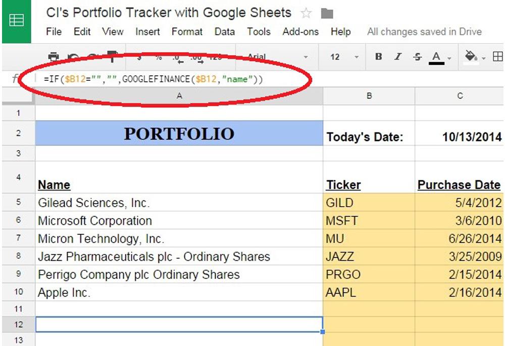
Without the IF function, you would see $0.00 in G5. Although this isn’t misleading, it is somewhat “cluttered” when the formulas are carried down throughout a blank spreadsheet. All calculated cells would display #INVALID_DATA, #ERROR or #VALUE until you input your holdings. You can see how this works by clicking on any blank cell under the column heading row. Each cell has the formula input already, so you don’t have to copy any formulas down the rows, and using the IF function keeps the cells blank until data is present. This is displayed in Figure 2.

The IF function is defined as:

=IF(logical_text, [value_if _true], [value_if_false])

If the logical text is determined to be true, then the “value if true” will result. If the logical text is determined to be false, then the “value if false” will result. In this case, if the referenced cell is blank (“ “), a blank should appear in the destination cell, and if the referenced cell is not blank, the formula after the final comma should be calculated in the destination cell.

Dollar signs are used in formulas to lock in a cell reference. When you copy and paste an Excel formula from one cell to another, the cell references change, relative to the new position. The “$” symbol is placed before the column reference to let Sheets know to change the row number when the formula is copied down, but not the column reference. This formula also applies to Microsoft Excel.

Column H is “Average Cost/Share.” The formula in cell H5 is as follows:

=IF($E5=““,”“,(($E5*$F5)+$D5)/$F5)

Again we are using the IF function to remove error messages when a purchase price hasn’t been input yet. The calculation multiplies your purchase price by the number of shares purchased, adds the commission fees and divides by the number of shares purchased to arrive at an average cost per share value.

Column I shows the market value of your holdings. The formula in cell I6 is:

=IF($A5=““, ““,($J5*$F5))

To prevent the error messages from appearing before the contents of cell A5 are input, the IF function is used. The market value is determined by multiplying the current price of the equity by the number of shares you purchased.

Column J contains the current price for each holding. Quotes may be delayed up to 20 minutes. The formula in cell J5 is:

=IF($A5=““,”“,(GOOGLEFINANCE($B5, “price”)))

The IF function was used again, but we also have a different type of formula in this cell. The GOOGLEFINANCE function tells the Google Sheet to pull data from Google Finance website. The syntax given by Google for Sheets is:

GOOGLEFINANCE(ticker, [attribute], [start_date], [num_days/end_date], [interval])

The first part of the formula requires the ticker symbol. In the example above, we substitute $B5 for “ticker” because each row will reference a different holding. So the sheet is programmed to reference cell B5 as the ticker in row 5 and B6 as the ticker for row 6, etc.

The “attribute” part of the syntax requires that users choose a specific attribute they are trying to access. Examples would be: price, high, low, volume, and market cap among other options. For a list of attributes and more information regarding them visit:

https://support.google.com/docs/answer/3093281?hl=en

The last three parts of the syntax are optional and they are not items that we use in this spreadsheet.

Column K displays the equity’s opening price for the day. The formula in cell K5 is:

=IF($B5=““,”“,(GOOGLEFINANCE($B5, “priceopen”)))

The IF function was used so ERROR values wouldn’t be displayed before a ticker symbol was input into the sheet. The GOOGLEFINANCE part of this formula references the ticker symbol in cell B5 and pulls in the data for the attribute “priceopen.”

Column L displays the intraday high corresponding to the ticker input in column B. The formula in cell L5 is:

=IF($B5=““,”“,(GOOGLEFINANCE($B5, “high”)))

The IF function was used to remove error values until a ticker was input in column B. Then the formula uses the GOOGLEFINANCE function by referencing the ticker symbol and the “high” attribute.

Column M displays the intraday low. In cell M5, you will see the formula:

=IF($B5=““,”“,(GOOGLEFINANCE($B5, “low”)))

The IF function was used to ensure that an error value wouldn’t be displayed if no ticker symbol is input into column B. Then the GOOGLEFINANCE function was used to return an intraday low figure once a value was input for the ticker in column B.

Column N displays the volume. In cell N5, you will see the formula:

=IF($B5=““, ““,(GOOGLEFINANCE($B5, “volume”)))

This formula uses the IF function to ensure that if no ticker has been input into the respective B column, no error will be displayed. Then the GOOGLEFINANCE function references the ticker in cell B5 and the attribute “volume.”

Column O displays a given equity’s 52-week high. In cell O5, you will see the formula:

=IF($B5=““,”“,(GOOGLEFINANCE($B5,”high52”)))

The IF function was used to prevent an error value from displaying if there is no ticker in the corresponding row. The GOOGLEFINANCE function references the ticker symbol in cell B5 and defines the attribute “high52,” or 52-week high.

Column P displays the security’s 52-week low. The formula in cell P5 is:

=IF($B5=““,”“,(GOOGLEFINANCE($B5,”low52”)))

The IF function was used to prevent error values from displaying before a ticker is input into the respective row. The GOOGLEFINANCE function references the ticker symbol in the row and provides a 52-week low figure.

Column Q provides users with the price-earnings ratio for a given security in their portfolio. The formula in cell Q5 is:

=IF($B5=““,”“,(GOOGLEFINANCE($B5, “pe”)))

The IF function was used to prevent an error value from displaying until the ticker symbol is input. If there is no ticker symbol, the cell will remain blank. The GOOGLEFINANCE function references the ticker symbol in column B for the row and then returns the “pe,” or price-earnings attribute.

Column R provides users with an earnings per share figure for a given ticker. The formula in cell R5 is as follows:

=IF($B5=““,”“,(GOOGLEFINANCE($B5, “eps”)))

The IF function was used to prevent an error value from displaying until the ticker symbol is input. If there is no ticker symbol, the cell will remain blank. The GOOGLEFINANCE function references the ticker symbol input in the corresponding row, and then returns an earnings per share figure.

Column S displays the daily change of a given security in terms of percentage. The formula in cell S5 is:

=IF($B5=““,”“,(GOOGLEFINANCE($B5, “changepct”)))

The IF function tells Google Sheets that if there is no ticker symbol in cell B5, then the cell S5 must remain blank. This prevents the cell from displaying an error message until we have input the necessary information. The GOOGLEFINANCE function references the ticker symbol in the corresponding row and then provides the attribute “changepct” to return a percentage change in price for the security since the previous trading day’s close.

Watchlist

The Watchlist tab of our portfolio tracker is where you can enter in stocks, mutual funds or ETFs that are on your radar screen, but are not part of your actual investment portfolio. When you click the Watchlist tab, you will see today’s date displayed at the top, along with three different indexes: the Standard and Poor’s 500 index, Wilshire 5000 Total Market Index (full cap) and the NASDAQ 100 composite. Columns C, D and E give the current price and daily change in terms of dollars and percent. Ticker symbols that users want to include on their watchlist are entered below the indexes in the cells highlighted in yellow. When ticker symbols are input into column A, all the corresponding columns will populate accordingly (Figure 3).

Figure 3. The Watchlist Tab

 

 

The Watchlist tab includes some of the same formulas from the Portfolio tab, except that the calculated cells reference column A for the ticker symbol instead of column B. However, there are a couple of formulas that weren’t included on the Portfolio tab: Current Price as % of 52-Week High and Current Price % Away from 52-Week Low.

In column N you will see the stock’s current price as a percentage of its 52-week high. The formula in cell N10 is as follows:

=IF($A10="", "", ($C10/$L10))

The formula uses the IF function to ensure that the cell will be left blank until a ticker symbol is input into cell A10. The second set of parentheses addresses the question, “What should the formula do if there is a ticker symbol input into cell A10?” In order to calculate what percentage the current price is of the 52-week high, we use a simple formula:

(Current Price)/(52-Week High Price)

For example, if a security’s current price is $94 and its 52-week high price is $123, $94 represents 76.4% of $123.

In column O you will see the stock’s current price compared to its 52-week low as a percentage. Cell O10 contains the formula:

=IF($A10="", "", ($C10/$M10)-1)

The IF function lets the formula know that if there is no value in cell A10 for a ticker, we want cell O10 to display a blank. Once the ticker symbol is input, then the formula will calculate how far away the current price is from the 52-week low price, using the formula:

(Current Price)/(52-Week Low Price)

Conclusion

CI’s Portfolio Tracker with Google Sheets is a simple and easy-to-use portfolio tracker that allows you to keep track of your current holdings as well as create a watchlist. This spreadsheet introduces users to Google Sheets, lets them know some of the functions and features that the program has to offer, and a free basic tool for investors. You can find plenty of further information regarding Google Sheets online.