First, a bit of background on this article along with some well-deserved acknowledgements. The AAII Silicon Valley Chapter’s Computerized Investing subgroup has been discussing Tactical Asset Allocation (TAA) strategies for multiple years. For much of that time if you wanted to try out different TAA ideas by backtesting them you had to either: a) do it yourself via downloading data, creating Excel formulas, coding equations, etc., or b) buy a simulation/backtesting tool to help you try out your idea.

Since 2013, a free, web-based tool—Portfolio Visualizer—has been available that eliminates much of this work. Consequently, much of our recent work on TAA has used Portfolio Visualizer.

Let me stop here and thank the creator of Portfolio Visualizer, Tuomo Lampinen, for providing this very powerful tool. Lampinen was kind enough to speak about Portfolio Visualizer at the AAII Silicon Valley Chapter in January of this year and it was quite rewarding and educational.

Let me make a few cautionary notes before we go further:

• Backtests can be over-tuned, leading to unrealistic results. There are a variety of ways to combat this exposure—for example, testing the strategy in different countries, testing with different instruments or doing out-of-sample testing. Other than mentioning the over-tuning exposure, this article does not delve into this aspect of backtesting.
• TAA always brings up the question of trading costs, primarily commissions and slippage. These costs are dependent on which brokerage you use, how you place your trades and many other factors. Given that this article focuses on highly liquid exchange-traded funds (ETFs), many of which may be free or low cost to trade, and that the frequency of trades usually isn’t more than monthly, many of the cost concerns are minimized.

TAA and Portfolio Visualizer: The Basics

TAA is a dynamic investment approach that actively adjusts a portfolio’s asset allocation with the goal of improving the risk-adjusted returns over passive investing. TAA uses shorter-term market expectations to take advantage of under- or overvaluation of securities, industries, sectors and asset classes. TAA differs from strategic asset allocation (SAA), which is often based on modern portfolio theory and focuses on selecting an asset allocation based on long-term expectations, historical correlations, returns and risk (usually as measured by standard deviation).

The TAA strategies we discuss here are widely known; two of them have books describing them and their associated performance (both backtested and real-time). The TAA strategies that we discuss include two relatively simple strategies and one more complex one:

• Dual Momentum (relatively simple)
• Target Volatility (relatively simple)
• Adaptive Asset Allocation (relatively complex)

As with any backtesting and analysis tool of this type, among the first questions you should ask yourself regarding Portfolio Visualizer are “Is the algorithm implementation correct?” and “How good is the data that is used?” Luckily, Portfolio Visualizer provides significant details to answer both of these questions on its FAQ page.

Tackling the question “Is the algorithm implementation correct?” first, the Methodology section of the FAQ provides several pages explaining how the various algorithms are implemented along with appropriate references. As an anecdotal check on the algorithm implementation, several members of our CI subgroup had already either implemented their own versions of these algorithms or had access to for-fee tools that performed these functions and found results of various test cases to match Portfolio Visualizer results. While not a complete check of Portfolio Visualizer’s implementation, these spot checks certainly build confidence that the implementation is correct.

Moving on to the question “How good is the data that is used?”, the various Data Sources sections of the FAQ again provide references and links to the data that is used. Even if you decide against using Portfolio Visualizer, the Data Sources sections are a gold mine of where to find free data if you are a dedicated do-it-yourselfer in this area.

Ultimately, the final question for the usage of any tool is “Do you trust it enough to invest your money with it?” This is, of course, a question that each of us must decide individually; my answer is “Yes”—I use Portfolio Visualizer regularly when making investment decisions.

With that, we’re now ready to start looking at TAA strategies as implemented by Portfolio Visualizer.

Dual Momentum

The Dual Momentum strategy was popularized by Gary Antonacci in his award-winning book “Dual Momentum Investing: An Innovative Strategy for Higher Returns With Lower Risk” (McGraw-Hill Education, 2014). Antonacci’s website, Optimal Momentum, provides a wide variety of information on this strategy. My comments here provide, at best, a basic introduction, but those wanting further information should visit the Optimal Momentum website.

At its most basic level, the Dual Momentum strategy is very straightforward in combining relative and absolute momentum checks to select the best asset or ETF out of the choices provided. The relative momentum check ranks the n-month gains of two or more assets/ETFs and picks the highest-ranked asset/ETF. An absolute momentum check is then performed where the winner(s) of the relative momentum race are compared to the risk-free asset (typically T-bills) over the same n-month period. If the relative momentum winner(s) outperform the risk-free asset then they are selected; if they underperform (e.g., by having a negative gain) then the risk-free asset is selected.

To demonstrate this within Portfolio Visualizer, we use the Global Equities Momentum (GEM) strategy. To illustrate GEM’s performance over an extended period, we use the Vanguard 500 Index fund (VFINX) to represent domestic stocks and Vanguard Total International Stock Index fund (VGTSX) to represent foreign stocks in our example. ETFs such as Vanguard Total Stock Market (VTI) and Vanguard Total International Stock (VXUS), or their equivalents at the brokerage of your choice, can also be used.

The setup for the Dual Momentum GEM strategy can be seen in Figure 1 below. Note that you can also see this strategy at Portfolio Visualizer by clicking here.

 

 

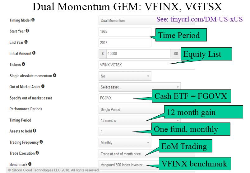
As you can see, the setup here is quite simple; only a few comments are required:

• Start and End Years: Here I defaulted to the maximum possible range starting in 1985. If one or more of your tickers does not have sufficient history for the range you have chosen, Portfolio Visualizer will truncate the time period to the shortest history ticker you provided. You can perform in and out of sample testing periods by adjusting the starting and ending periods appropriately.
• Out of Market Asset: I chose Fidelity Government Income fund (FGOVX) as a relatively safe alternative that provides reasonable gain; your choice may differ based on your risk level and available ETFs and mutual funds.
• Performance, Timing Periods: I chose a single period of 12 months to stay true to the GEM strategy, but Portfolio Visualizer allows many more options.
• Trading Frequency, Execution: Portfolio Visualizer allows several choices of trading frequency, in this case weekly to quarterly. After a bit of experimentation, you may find that trading more frequently does not help your performance! With respect to trading execution, Portfolio Visualizer allows you to choose making trades on the close at the end of the trading month or at the close of the day after the end of the month. This allows adapting to how and when you make your trades.

Portfolio Visualizer provides a rich set of output screens after it completes. The examples below show some key output results—there are many others. Again, feel free to explore and choose those that best meet your needs.

 

 

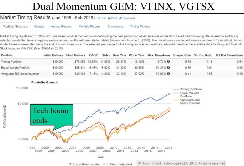
Figure 2 illustrates the summary statistics that Portfolio Visualizer provides—including initial and final balances, compound annual growth rate (CAGR), maximum drawdown (MDD) and Sharpe and Sortino ratios. Note that, under the Metrics tab, Portfolio Visualizer provides an even richer set of statistics. Portfolio Visualizer also generates the equity curves for the Dual Momentum algorithm, an equal-weight portfolio and your chosen benchmark (in this case the VFINX). Due to the extended time frame and large gains involved, we selected a semi-logarithmic scale to more accurately represent the performance of the three results. (Note: Semi-log scales are used since compound growth rates appear as straight lines when plotted on these charts.)

With respect to the results of the Dual Momentum GEM strategy, you can see that it put up quite respectable results in the CAGR, standard deviation and Sharpe ratio areas. The equity curves allow you to see that much of this outperformance was accomplished by avoiding the very large losses that occurred during the 2002–2003 and 2008–2009 bear markets; the absolute momentum check gets credit for this performance. However, no algorithm is perfect; you can see that Dual Momentum missed out on the sharp recoveries from those bear markets in the latter parts of 2003 and 2009.

Figure 3 below shows the drawdown curve for this Dual Momentum example.

 

 

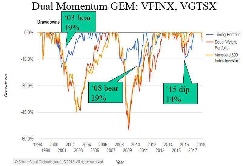
I find that the drawdown curve is one of the most important curves for any investment choice. Why? It provides a visual representation of the pain an investor must live through for any given investment strategy. Here you can see that both the Equal Weight and S&P 500 benchmark portfolios experienced roughly 45% drawdowns in the 2002–2003 bear and over 50% drawdowns in 2008–2009. Very few investors can open their brokerage statement, see that they have lost near or over 50% of their investment (admittedly, on paper) and carry on as normal. In fact, I believe that drawdowns are the source of much of the individual investor phenomena of “selling low and buying high.” Most investors simply cannot psychologically tolerate the pain involved when they see their hard-earned savings shrink by too large a percentage, so they choose to sell—realizing the loss—to stop the pain.

The Dual Momentum GEM algorithm did quite well with respect to drawdowns, experiencing “only” 19% drawdowns in the two bear markets. Note, however, that Dual Momentum saw a 14% drawdown in the 2015–2016 market dip; this was not appreciably different from the S&P 500 benchmark. The lesson here is not that Dual Momentum (or for that matter any algorithm) will magically protect you from all market drawdowns; however Dual Momentum has a respectable track record of protecting investors from significant, major market drawdowns.

Moving on to our final illustration for this algorithm, Figure 4 below shows the trades executed during the backtest.

 

 

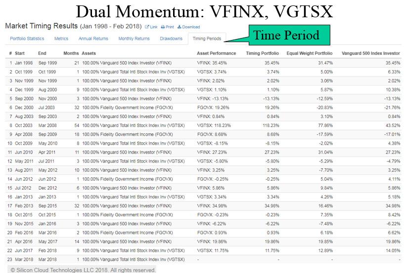
Figure 4 shows the complete history of trades made during the backtest period as well as the performance of the Dual Momentum, Equal Weight and S&P 500 benchmark portfolios. As Figure 4 shows, there are long time periods when the Dual Momentum algorithm stays in the same asset/ETF. Examples of this include the 18-month period from April 2008 to September 2009 that the portfolio was in Fidelity Government Income Fund (FGOVX), the 54-month period from October 2003 to March 2008 when it was in Vanguard Total International Stock Index Fund (VGTSX) and the 32-month period from February 2012 to September 2015 when it was in Vanguard 500 Index Fund (VFINX). Finally, at the end of each month, this output can be reviewed to determine which asset/ETF to be in for the coming month. For example, the last entry in Figure 4, for March 2018, shows a continued position of holding VGTSX.

Some closing thoughts on Dual Momentum at Portfolio Visualizer:

• Dual Momentum is a wonderful example of a straightforward algorithm that produces good performance. Dual Momentum does not have tons of assets/ETFs, complex mathematical analysis, multiple “moving parts,” etc. This simplicity and straightforwardness lends greatly to its credibility.
• Of course, given the capabilities that Portfolio Visualizer provides, there are several ideas and “What if?” scenarios that many will be interested in trying out. Examples include market-cap size experiments [small-medium-large such as Vanguard Small-Cap Index Fund (NAESX), Vanguard Mid-Cap Index Fund (VIMSX) or Vanguard 500 Index Fund (VFINX)], regional experiments (U.S.-Europe-Pacific) and sector experiments (e.g., picking the top three to five sectors out of the 10 SPDR sector funds).

Target Volatility

Algorithms that target a volatility level dynamically adjust the weight of one or more equity assets/ETFs against one or more bond-cash assets/ETFs to achieve the target volatility. In the case of Portfolio Visualizer, the adjustment is done based on historical volatility of the assets/ETFs looking backward over some number of months. Thus, when the market is volatile, such as during late 2008 and early 2009, the equity/ETF weighting is reduced; during calm periods such as most of 2017, the equity/ETF weighting is increased. I like to think of this strategy as a “dynamic growth and income fund” or perhaps a “dynamic 60/40 fund” where the 60/40 ratio varies based on current market volatility.

To demonstrate Portfolio Visualizer in this area, we use an extremely simple mix of ETFs: the S&P 500 as represented by VFINX and a generic bond fund as represented by FGOVX. Those who believe that bond funds are a poor selection to use in the current rising rate environment can substitute cash, or very short-term bond funds, instead. There is an argument that bond funds may still be superior to cash in a market that has rising volatility—but that argument can be held another time.

The setup for the Target Volatility strategy can be seen in Figure 5 below. Note that you can also see this strategy at Portfolio Visualizer by clicking here.

 

 

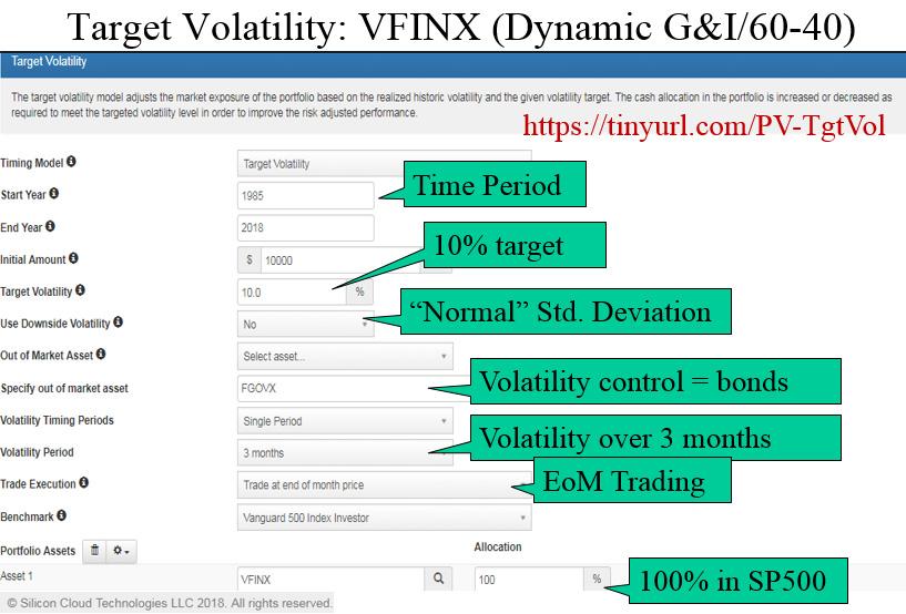
Again, the setup here is quite simple, with only a few comments needed:

• Start and End Years: Here we defaulted to the maximum possible range starting in 1985. If one or more of your tickers does not have sufficient history for the range you have chosen, Portfolio Visualizer will truncate the time period to the shortest history ticker you provided.
• Target Volatility: We picked 10% which is (very roughly) two-thirds of market volatility over long periods and is also (very roughly) the volatility you may see in a 60/40 balanced fund.
• Use Downside Volatility: Roughly speaking, downside volatility calculates volatility based only on the days the market is down. The theory here is “Who cares how volatile the market is if it’s going up?” Our setting is “No,” which allows both up and down market days to participate in the volatility calculation.
• Out of Market Asset: We chose Fidelity Government Income Fund (FGOVX) as a relatively safe alternative that provides reasonable gain; your choice may differ based on your risk level and available ETFs/mutual funds.
• Volatility Timing Periods: We chose a single period of three months to be somewhat reactive to the market but not overly so. In my own studies, I have found three months to be a good compromise between very short-term periods (one month) and very long-term periods (one or more years). You can certainly find support in industry and academic papers for other periods. Experimenting with different time periods can be fun.
• Trading Execution: As before we chose to make trades on the close at the end of the trading month.

Figure 6 below provides the summary statistics and equity curves for the backtest.

 

 

With respect to the results of the Target Volatility strategy, you can see that it put up quite respectable results in the standard deviation, Sharpe ratio and max drawdown areas. (Note that the standard deviation is below the 10% target.) The CAGR is competitive with a buy-and-hold the S&P 500 strategy. The equity curves allow you to see that much of this outperformance was again accomplished by avoiding the very large losses that occurred during the 2002–2003 and 2008–2009 bear markets. However, this algorithm has its drawbacks as well; at the height of the tech boom in the summer of 2000, your results were only 70% of the buy-and-hold S&P 500 strategy. Of course, you were not subjected to the large drawdown seen in 2002 and early 2003. Keeping in mind the goals behind the Target Volatility strategy and the simple mix used, I would submit that the algorithm did well over this period.

Figure 7 below shows the drawdown curve for this Target Volatility example:

 

 

Here again you can see that the S&P 500 benchmark experienced roughly 45% drawdowns in the 2002–2003 bear market and over 50% drawdowns in 2008–2009. Additionally, since we have a longer backtest history, you can see that the Black Monday event caused a 30% drawdown at month end while the Target Volatility strategy saw a 17% drawdown. Also, note that the target volatility strategy only saw a roughly 7% drawdown during the recent sharp drops in late 2015 and early 2016.

Moving on to our final illustration for this strategy, Figure 8 below shows the trade history since 2016.

 

 

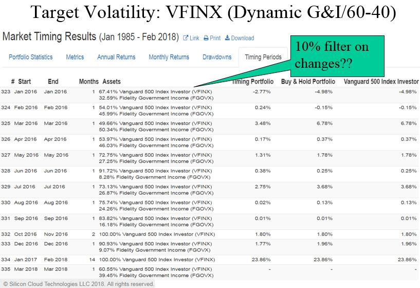
Figure 8 shows the trade history since 2016 and the performance of the Target Volatility (S&P 500) portfolios. Except for the period from January 2017 through February 2018—when the market was so calm that you could stay 100% in the VFINX (S&P 500 index) for 14 months straight—the algorithm rebalances every month as it adjusts to the market conditions. A few comments on this:

• There are those who will not like trading this frequently; one option is to apply a “10% change” filter—where the ETF weights must change by 10% or more to make a trade—to cut down on the trading frequency.
• With many mutual funds and ETFs allowing monthly trading for free, and the liquidity of ETFs like SPDR S&P 500 (SPY) or iShares Core U.S. Aggregate Bond (AGG) leading to miniscule spreads, I am not overly concerned with trading costs.
• Trading this frequently would certainly lead you to want to implement this algorithm in a tax-deferred account, as frequent trading in a taxable account reduces returns and increases costs.

Some closing thoughts on experiments you may want to try with the Target Volatility strategy:

• The trade-offs between high and lower volatility targets, as well as longer and shorter time periods over which to calculate volatility, may provide some insights.
• Repeating the experiment with more volatile ETFs—e.g., Invesco QQQ Trust (QQQ) and iShares 20+ Year Treasury Bond (TLT)—provides a bit more “punch” to the results.

Adaptive Asset Allocation

For our final example of Tactical Asset Allocation at Portfolio Visualizer we will explore the Adaptive Asset Allocation (AAA) strategy as described by ReSolve Asset Management. The AAA strategy has been popularized by Adam Butler, Michael Philbrick and Rodrigo Gordillo of ReSolve in their book “Adaptive Asset Allocation: Dynamic Global Portfolios to Profit in Good Times—and Bad” (Wiley, 2016). The basics of the AAA strategy can be found in the paper “Adaptive Asset Allocation: A Primer.” Once again, my comments here provide, at best, a basic introduction to these concepts; please refer to the paper and book for further detail.

While the details of the AAA can be quite complex, at its simplest the AAA strategy breaks down into three parts:

1. Selecting a suitably broad set of assets/ETFs, a subset of which should do well in any market environment,
2. Selecting a relative strength algorithm that will rank the assets/ETFs chosen and pick the top “N” assets/ETFs and
   
3. Selecting a weighting algorithm that weights the selected top “N” assets/ETFs appropriately. We use an example of AAA at Portfolio Visualizer to provide further detail on each of these parts.

The setup for the AAA strategy can be seen in Figure 9 below. Note that you can also see this strategy at Portfolio Visualizer by clicking here.

 

 

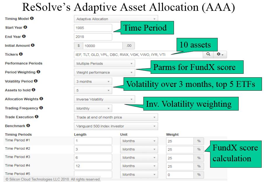
Here the setup of the strategy is a bit more complex; the details of what was chosen and why are given below:

• Start and End Years: Once again, we defaulted to the maximum possible range starting in 1985.
• Tickers: As mentioned above, for AAA to work it must have a suitably broad set of assets/ETFs, a subset of which should do well in any market environment. For the purpose of this backtest, the universe of 10 ETFs we chose includes these ETFs: iShares 7-10 Year Treasury Bond ETF (IEF), iShares 20+ Year Treasury Bond ETF (TLT), SPDR Gold Shares (GLD), Vanguard FTSE Pacific Index (VPL), Deutsche Bank Commodity Index (DBC), SPDR Dow Jones International Real Estate Index (RWX), Vanguard FTSE Europe Index (VGK), FTSE Emerging Markets Index (VWO), iShares U.S. Real Estate Index (IYR) and Vanguard U.S. Total Stock Market Index (VTI).
• Performance and Timing Periods: For the relative strength algorithm, we chose to use a slightly modified version of the FundX score developed by NoLoad FundX. Here we equally weight the one-, three-, six- and 12-month gains to come up with the modified FundX score. This is shown in Figure 9 in the “Parms for FundX score” and “FundX Score calculation” callouts.
• Volatility period: As before, we again chose three months to be somewhat reactive to the market but not overly so.
• Assets to Hold: Here we chose to hold the top five of the 10 ETFs provided. Based on past backtesting work I have done, I find that it is best to hold the top 25% to 50% of the ETFs available to you.
• Allocation Weights: Here Inverse Volatility was chosen. Inverse Volatility provides greater weight to those ETFs that have lower volatility. For example, if you have ETFs A and B, and B is twice as volatile as A, Inverse Volatility will result in ETF A being twice the weight (67%) of ETF B (33%). Beware that one of the often-unexpected results of Inverse Volatility weighting is that if a very low volatility ETF is used—e.g., Barclays 1–3 Month T-bill (BIL)—almost all of your funds will be placed in that ETF since it is of extremely low volatility.
• Trading Execution, Frequency: As before, we chose to make trades on the close at the end of the trading month.

Figure 10 below provides the summary statistics for the AAA backtest.

 

 

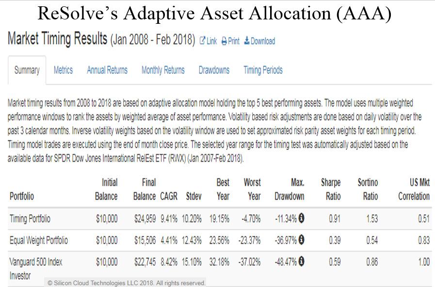
With respect to the results of the AAA strategy, the first thing that must be noted is the relatively short backtest time period of only 10 years, which is caused by the relatively short history of RWX. This period only covers one bear market and recovery and a unique period that includes a financial crisis, quantitative easing and many other unusual items. Given that proviso, you can see that AAA put up quite respectable results in the CAGR, standard deviation, Sharpe ratio and max drawdown metrics. This outperformance is mainly due to the AAA strategy becoming heavily weighted in IEF, TLT, GLD and non-equity ETFs in the latter half of 2008 and the first quarter of 2009.

Figure 11 below shows the equity and drawdown curves for this AAA example.

 

 

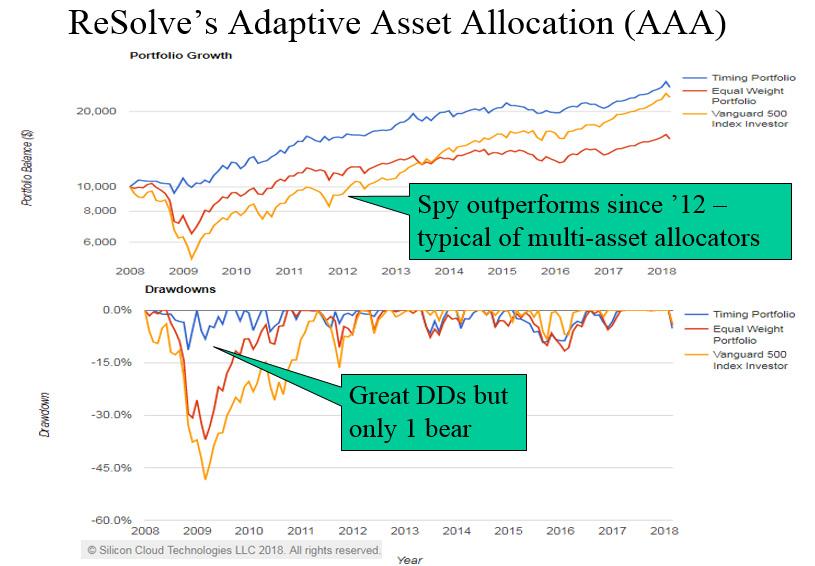
The equity curves in the upper panel of Figure 11 show that AAA’s outperformance was again accomplished by avoiding the very large losses that occurred during the 2008–2009 bear market. However, since 2012, the Adaptive Asset Allocation strategy, like many multi-asset allocation strategies, has suffered when compared to the S&P 500’s performance. Put simply, when you are forced to hold several assets/ETFs it is hard to beat the top-performing asset/ETF!

Reviewing the drawdown curve, you can see that the maximum drawdown occurred in October 2008; the market dip we experienced in late 2015/early 2016 caused less than a 10% drawdown to occur in the AAA strategy.

Next, we move on to our final illustration for AAA; Figure 12 below shows the trade history since December 2017.

 

 

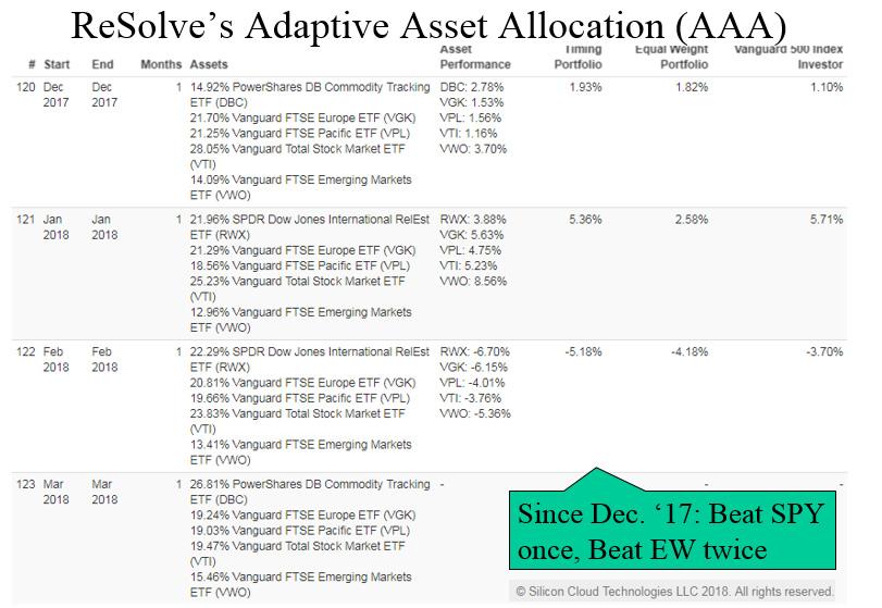
As in the Target Volatility strategy, Figure 12 shows that the Adaptive Asset Allocation strategy rebalances every month as it adjusts to changing market conditions—consequently, it faces many of the same drawbacks and criticisms:

• AAA faces significant criticism with respect to frequent trading and the overall number of trades needed; one option is to again apply a “noise trade” filter of perhaps 5%–10% to cut down on the trading frequency. Without such a filter 120 trades per year should be expected (though many of these will be relatively small changes in existing position sizes).
• While most of the ETFs in the chosen universe are large and should not suffer from any significant spread costs, there may be commission and other trading costs in some of these ETFs depending on your brokerage of choice.
• Trading this frequently would certainly lead you to want to implement this algorithm in a tax-deferred account.

Below are some closing thoughts on variations that you may want to try with the AAA strategy. But be forewarned, there are many “knobs you can turn” on the AAA strategy and over-tuning can easily result in unachievable results in the real world.

• The universe of ETFs can be varied to reflect the best ones for you/your brokerage. Also, the number of ETFs to be chosen each month can be varied, with the ranges mentioned above providing guidance on reasonable limits.
• All of the AAA parameters—the relative strength algorithm, volatility lookback period and weighting algorithm, the number of ETFs to be held—can be varied as you see fit. (Remember my caution on over-tuning!)
• If you are particularly adventurous, and have a lot of time on your hands, you can run AAA multiple times with various relative strength algorithms, volatility lookback periods and weighting schemes that individually seem reasonable to you. Taking an average of all these weights should reduce the possibility of over-tuning to any specific set of parameters.

Summary

We started this article by reviewing the painful process that historically an individual investor had to go through to backtest and analyze a TAA strategy and how Portfolio Visualizer frees the individual investor from the drudge work involved in that effort. We discussed both the data and algorithms Portfolio Visualizer uses. To illustrate how Portfolio Visualizer can be used to study TAA, we walked through the setup and backtest results of three TAA strategies, two (Dual Momentum and Target Volatility) that were relatively simple and one (Adaptive Asset Allocation) that was relatively complex.

Throughout the article I provided a number of references to books and websites that you can use to investigate items further. Hopefully, I have convinced you that Portfolio Visualizer is a reasonable tool to use and that the information here can help you get started backtesting, analyzing and ultimately implementing the TAA scheme of your choice. Good hunting, and by all means enjoy yourself!