To construct an optimal portfolio for any investor requires knowledge of two quite different types.

Most obviously, we need to have some knowledge of investments: What is the expected risk and return of all the assets we could use to build the portfolio, and to what degree are they likely to rise or fall together? Secondly, if we are to succeed in combining these into optimal portfolios, we need to understand investors: In particular, we need to know exactly what trade-offs between risk and return each investor is prepared to make. Without this knowledge we may well design a portfolio that is optimal ... but optimal for whom?

The core model used by the financial services industry to construct optimal portfolios of risky assets, known as modern portfolio theory (MPT), was developed almost 60 years ago. This model embodies a number of brilliant insights, still relevant today, about how investors should combine assets in an efficient way to simultaneously reduce expected risk and maximize expected return to attain a portfolio that displays the optimal trade-off between the two for each individual investor. However, 60 years ago our state of knowledge was considerably lower than it is today, in many crucial areas:

Our access to investment data was far poorer than it is now: There were fewer asset classes than there are today, and we were at a time of stable growth. As such, we knew vastly less about the dynamics of all asset classes and investments.

Decision science, and in particular behavioral finance, was not even in its infancy: We had to rely on what are now, and were then, recognized to be extremely simplistic models on how real investors think about and trade off risk and return.

Finally, in the early 1950s we were in a world almost completely without modern computing power. All optimization calculations had to be done by hand using inputs from existing, and frequently hard-to-access, data: The rules had to be simple and intuitive, even if this meant knowingly sacrificing some realism in favor of tractability.

In short, not only does MPT make outdated and simplistic assumptions about both investors and investments, but also whatever justification there was for sticking with these assumptions on the grounds that they made calculation of the solutions simpler has also significantly disappeared. The last nail in the MPT coffin came with the realization at the end of the 2000s that a portfolio driven by modern portfolio theory would not outperform a portfolio based simply on an equal allocation across assets.

It is time to revisit MPT in the light of what we know today and to ask how the advances of the last half century change the solutions that the financial services industry has been clinging to for so long. It is also time to link updated techniques and the search for performance.

This is the task we set ourselves in our book, “Behavioral Investment Management” (McGraw-Hill, 2012). We ask both how our model of investors’ long-term preferences should be updated with the advent of behavioral finance, and how we can more accurately measure our expectations of the future returns of all investments.

Modern Portfolio Theory: The Classical Model

Figure 1 illustrates the principles of the existing model of modern portfolio theory. It shows how we can articulate the essential trade-off between the expected risk and return of all investments by placing them on a risk-return chart. Each black dot represents a particular investment in risk/return space. Clearly, investors should prefer to have higher returns and lower risks. MPT tells us how to calculate the efficient frontier—the curve that exhibits the most efficient possible combinations of all available assets (given our knowledge of them) such that for any given level of risk we have the portfolio with the highest possible return. The efficient frontier makes full use of the diversification benefits of combining assets together so that we minimize the risks to the overall portfolio with the minimum possible sacrifice of the overall return.

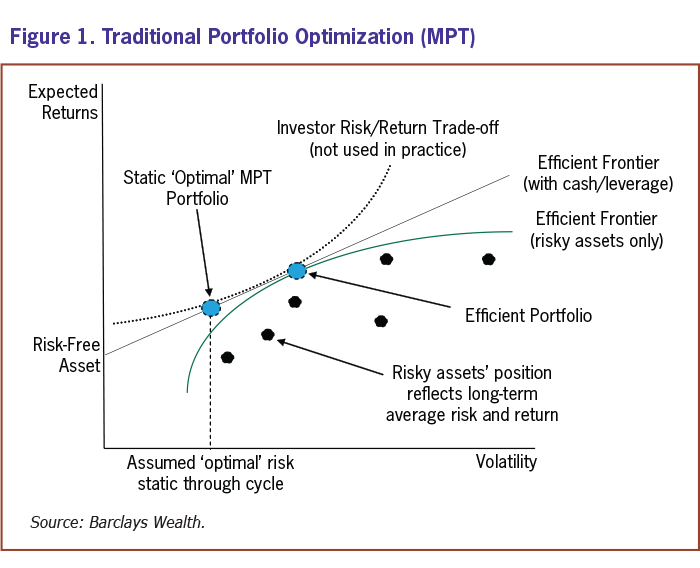
On this curve is a single portfolio that provides us with the most efficient trade-off between expected risk and return. Of course, this portfolio is not perfect for everyone. Some people have lower tolerance for risk and so should be in a less risky portfolio. Some are more willing to take risk and so should have a more risky portfolio. But in MPT, the best solution for all investors can be achieved either by mixing the efficient portfolio with cash for safer portfolios or by leveraging to take on more risk. These combinations are shown by the straight line connecting the risk-free asset (100% cash) with 100% of the efficient portfolio and beyond (leveraged portfolios).

The last component is achieved by drawing a line that best reflects the risk/return preferences of each individual investor. All investors should be prepared to accept a little more risk, as long as the rewards are high enough. But risk-averse investors will require a greater expected return to accept any increase in risk, while others will quite readily take on more risk in the quest for greater expected returns. An example of such a curve is shown as a dotted line on the diagram: As risks increase, this investor will require ever greater expected returns as compensation.

This setup looks in principle extremely powerful, and the model ensures that investors have portfolios that make the most effective use of the risk that they are prepared to accept to turn this into higher expected returns. But in practice, a great deal depends on how we measure the original risk and return of each investment and also on how we determine the trade-off between overall risk and return that is optimal for each investor. And this is where MPT is mired in the past. Both the efficient frontier and the indifference curve representing investor preferences are calculated using quite unreasonable assessments, of investments in the first case and of investors in the second. Let’s look at each in turn.

Understanding Investors

It is a difficult task to determine exactly what long-term trade-offs between risk and return should be optimal for investors. Indeed, because of our lack of robust behavioral knowledge, the line representing investor preferences has typically been left out of practical applications entirely. Instead, the financial services industry has simply made arbitrary assumptions about what level of risk is optimal for each investor (e.g., 8% volatility for a moderate-risk-tolerance investor), regardless of market conditions, and then simply used the efficient frontier to determine the portfolio with the best expected returns for that level of risk.

This means that, while we may identify the expected risk level of all portfolios offered to investors, we really have no way of claiming that these are the best combinations of risk and return at any point in time. Why, for example, should 8% volatility be the right level for a moderate-risk investor, regardless of market conditions? Surely in times when the rewards for taking risk are higher, we should aim for portfolios that target slightly higher risk, and when the expected returns to risk are lower, we should decrease risk. To really ensure that portfolios are optimal for investors, we have to know how to draw the lines reflecting their risk and return preferences.

The problem is that we can’t determine this line by looking at the real behavior of investors. Every decision is made in the present, even if it is intended to achieve long-term outcomes. Our real decisions, then, are frequently not particularly accurate reflections of long-term risk/return preferences: They are clouded by all manner of emotional responses and behavioral distortions. Even though experimental economists have become very skilled at modeling our short-term decisions, the last thing we should be doing is using these as the basis for supposedly ‘optimal’ portfolios. We would simply end up replicating all the emotional decision biases that harm investors’ long-term performance.

Fortunately, however, rather than replicate biases, we can use our knowledge of behavioral decision science to ‘clean’ the preferences of these undesired short-term distortions. These techniques allow us to draw the lines reflecting clean, rational, risk and return preferences for investors of any level of risk tolerance, as long as we are prepared to make a small but significant change to the diagram: We have to change what we mean by ‘risk.’

What Is Risk?

In MPT, when people speak of risk, they typically mean annualized standard deviation of returns—or volatility, as it is frequently called. [Standard deviation measures the extent to which returns have historically varied; the larger the standard deviation, the greater the magnitude by which returns have fluctuated both to the upside and to the downside.] Although it is (relatively) simple, there are two big problems with volatility as a risk measure. Firstly, it doesn’t completely measure the full risk of investment returns. There has been a lot in the last few years about “black swans” and other extraordinary events. Volatility only captures the high-frequency/low-incidence deviations from the expected value, which only fully characterize unexpected outcomes in the case of bell-shaped, normally distributed returns (which would be handy, but is rarely the case in practice). Standard deviation does not do a good job of measuring the risk of events that are far different from the expected norm (called “tail events”). And it’s these events that are most important to investors when considering risk, which brings us to the second problem.

We should want a measure of risk to reflect what really matters to investors. After all, in the optimization process we’re going to be actively trying to reduce ‘risk,’ so the measure that we’re trying to reduce should only reflect outcomes that are intuitively held to be ‘bad’ to real investors. So how does volatility fare on this standard? Again, the answer is, badly. Volatility is a symmetrical measure. It counts as ‘risk’ any deviations from the mean, whether they are negative or positive. This is completely contrary to intuitive notions of ‘risk,’ which should be about the chance of bad things happening. When we choose a measure of ‘risk’ that defines what we’re trying to minimize in portfolio optimization, it is simply not good enough to accept a measure that means we penalize good outcomes along with the bad.

The idea here is to depart from a setup that is purely driven by the focus on mathematical simplification and stylization and to look at individuals. Fortunately, it turns out that defining a behaviorally ‘cleaned’ long-term preference for risk and return has, as a useful by-product, an alternative measure of risk, which does not suffer from the same weaknesses. We call it behavioral volatility. A particularly nice feature of behavioral volatility is that, where the returns are normally distributed (and therefore completely symmetrical), behavioral volatility and regular volatility are exactly the same. But when the distribution is skewed negatively, behavioral volatility is higher than its traditional sibling, reflecting the fact that investors should dislike these two features of investment returns. This provides us with the tantalizing possibility of a risk measure that can consistently compare any two investments, no matter how non-normally returns are distributed.

A second, very fundamental, difference is that risk measured by behavioral volatility becomes subjective. Different investors, with different degrees of risk tolerance, may value risk differently for the same investment. This is because investors who have low risk tolerance should also have greater aversion to a sharp decrease in asset values than less-risk-averse investors, and should thus penalize investments with these features to a greater extent. Intuitively, this makes complete sense: Something can only be risky insofar as it is risky for someone, and people are different.

Understanding Investments

There are two primary advances on MPT in how we approach the formation of the efficient frontier. The first follows from the discussion above: The frontier shows the best possible expected returns for each level of risk. Each investor wants to minimize the risk that is meaningful to them. But when we accept that risk must be subjective, the efficient frontier must be too. Where all assets are normally distributed and symmetrical, there will be no differences either in risk between investors or in the shape of the frontier.

The other, more important, upgrade to the efficient frontier is that it has to be dynamically adjusted. The economic environment is constantly in flux. The interesting point though is that, according to robust academic findings, it is more relevant to say asset prices alternate between periods of growth and losses than to say that they follow a pure random walk. The best way to characterize this is to speak about regimes—i.e., altering periods of asset price growth and of asset price losses. As the world oscillates between these states, it is impossible to argue that our expectations for the risk and return of investment assets should remain constant. And yet this is precisely what is implicit in conventional uses of the efficient frontier. In a turbulent world, being right on average means being wrong most of the time. The classical efficient frontier is periodically accurate in much the same way that a stopped clock is exactly right twice per day.

Instead, part of the process is to uncover which regime we tend to be in, in order to be able to adapt to these changing market conditions sufficiently early. The idea is not to forecast turning points, a very challenging undertaking, but rather to capture these turning points rapidly once they have taken place. The extremely interesting feature is that instead of looking at the dynamics of asset prices through the prism of normality and periodic accidents, we move to a more mature approach where within a regime the asset dynamics are well behaved, but shifts from one regime to another take place five to 10 times every decade. In this framework, our objective is to adapt the efficient frontier to the regime we find ourselves in.

Our approach to drawing a dynamically evolving efficient frontier involves a) measuring risk with behavioral volatility, so it’s meaningful to the investor, and b) measuring the expected risk and return of assets dynamically and frequently, using nimble estimation techniques so they’re meaningful for the current economic regime. In total, this means that the frontier is in flux as assets’ risks and expected returns regimes change. This means being much more responsive to recent data than the traditional model suggests. With frequent rebalancing and nimble portfolios, the weight of evidence tells us that it is better to miss the turning point but then adjust quickly than to be chasing a mythical ‘average’ regime throughout the economic cycle.

Combining the Two for Optimal Investment

The dynamic nature of the efficient frontier brings us to the final advance of behavioral investment management, illustrated for a good regime in Figure 2 and for a bad regime in Figure 3. We have used a better understanding of investors to redefine, for each investor, the optimal trade-off between risk and return to match long-term preferences, as well as the measure of risk itself. We have used this improved risk measure, and a dynamic regime-based view of investments to improve the accuracy of the efficient frontier at any point in time. Each of these innovations, on its own, adds to the risk-adjusted performance of the optimal portfolios. However, it is when our enhanced models of investors and investments are combined that we truly reap the benefits of the overall model.

Improving our understanding of investor preferences is of positive but limited use if the efficient frontier we use fails to accurately reflect the risks faced by the investor and is static throughout the cycle. Similarly, a dynamic regime-specific efficient frontier gets us to a set of portfolios more appropriate to the environment, but we won’t be able to make full use of this without a model of how investors should optimally trade-off risk and return in this changing environment. We’ll be forced to always pick the portfolio with a constant risk level, whereas investors should also be dynamically adjusting their risk levels as the environment shifts. Figures 2 and 3 show schematically how these changes to MPT will help investors reap the full benefits of dynamically optimal portfolios in a changing world. In the ‘good’ regime (Figure 2), the efficient frontier is higher, reflecting better expected returns, and the optimal portfolio reflects the optimal risk-return trade-off for the investor, not just the best returns for a fixed level of risk. In the ‘bad’ regime (Figure 3), the model adapts to the low-return environment: The efficient frontier is lower, and the investor shifts to a far less risky optimal portfolio.

Conclusion

Modern portfolio theory in its original form contained some deep and valuable insights. But it led to a static model that neither reflected risk as it matters to real investors, nor adapted to a constantly fluctuating world.

By updating the model to reflect our hugely increased understanding of both investors and investments, we can retain the essential insights that have proved so valuable in portfolio theory, while ensuring the model produces dynamically optimal results for individual investors, regardless of their risk tolerance.

Related

Beginning Investor

The Benefits of Modern Portfolio Theory