


Related

Financial Planning
This hybrid approach adjusts withdrawals within preset limits, allowing retirees to benefit from good markets and more easily weather bad markets.

This article was adapted from the authors’ September 2016 Vanguard research paper “From Assets to Income: A Goals-Based Approach to Retirement Spending.”
A number of spending rules—each emphasizing different goals—have been developed to help retirees deal with changes in their individual circumstances and in the markets.
Each rule places different emphasis on the competing priorities that many retirees are trying to balance: maintaining a relatively consistent level of current spending; and increasing—or preserving—the value of a portfolio to support future spending, bequests, and other goals. Two of the most popular rules are the dollar plus inflation rule (one example of which is William Bengen’s 4% spending rule) and the percentage of portfolio rule. While these rules of thumb are used by many, they may not be flexible enough to provide a tailored solution for each retiree’s unique circumstances.
To provide a customized solution for each retiree, we suggest a hybrid of these two rules, which we call the “dynamic spending” rule. With this rule, annual spending is allowed to fluctuate based on the performance of the markets, while at the same time being sensitive to significant fluctuations in spending from year to year. This is accomplished by overlaying an annual ceiling and floor to each year’s spending amount. As discussed in more detail in this article, the outcomes are significantly affected by the selection of the ceiling and floor percentages; this is where retirees, and their advisers, can tailor the strategy to provide the flexibility each retiree needs to meet his or her unique goals.
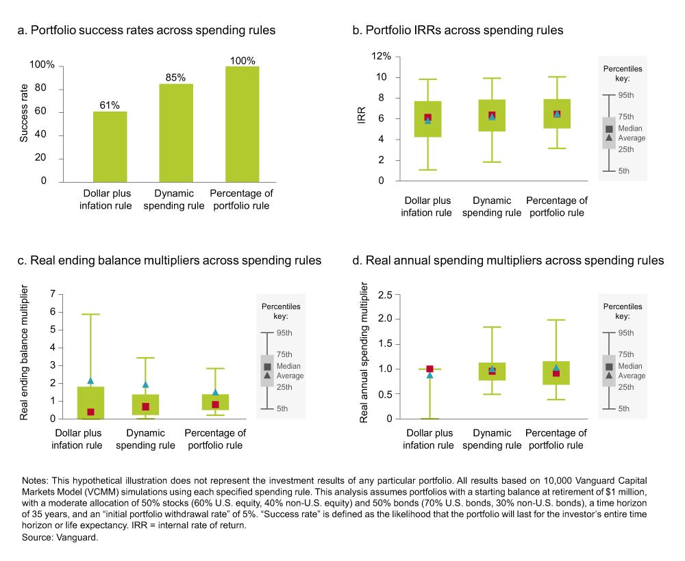
We prefer to see these spending rules as a spectrum of choices based on the relative importance a retiree places on each of their goals. Thus, at one end of the spectrum is the dollar plus inflation rule, which is essentially the dynamic spending rule with a 0% ceiling and a 0% floor. At the other end of the spectrum is the percentage of portfolio rule, which is essentially the dynamic spending rule with an unlimited ceiling and unlimited floor. The dynamic spending rule is positioned in the middle of these two rules in terms of potential outcomes. Figure 1 highlights the trade-offs of each rule more specifically.
For a retiree whose primary goal is spending stability, the dollar plus inflation rule (dynamic spending rule with a 0% ceiling and 0% floor) would likely be preferred. With this rule, upon retirement, a retiree selects the initial dollar amount he or she wants to withdraw from the portfolio in the first year and then increases that sum by the amount of inflation each year thereafter. Although this rule allows for more stable spending from year to year than the other spending rules we discuss, it comes with the risk of either premature portfolio depletion or lifetime under-consumption. This is because the strategy is exposed to sequence of returns risk; that is, it is indifferent to the capital markets, given that the annual spending amount is automatically increased by inflation regardless of whether the portfolio’s market returns are positive or negative. A significant period of market underperformance without an adjustment in spending could result in the retiree running out of money before the end of the investing time horizon. Conversely, a significant period of market outperformance could provide a retiree the opportunity to increase spending if desired. Failure to appropriately tailor spending to market performance could thus mean a retiree either misses out on enjoying retirement to the fullest extent possible or, at the other extreme, overspends and depletes the portfolio too soon.
At the other end of the spectrum, for a retiree whose primary goal is not depleting the portfolio, the percentage of portfolio (dynamic spending rule with an unlimited ceiling and unlimited floor) would likely be preferred. With this rule, a retiree annually withdraws a fixed percentage of his or her portfolio balance so that the annual spending amount is automatically increased or decreased based on the markets’ performance; this rule is thus highly responsive to the capital markets. Although the retiree’s portfolio will not be depleted (even though the spending amount may be substantially reduced through time), the annual spending amount can fluctuate significantly, which may not be an option for retirees whose nondiscretionary or fixed expenses (such as housing or food) are a relatively high proportion of their total expenses. However, for those with very high, if not unlimited, levels of flexibility, this option may be preferred. [For simplicity, we based the percent of portfolio spending amounts on annual ending balances. In practice, it is common to apply three-year smoothing to the percent of portfolio strategy, which would generate similar results (directionally) to those presented here; however, the variance would be truncated.]
Figure 1. Comparison of Various Spending Rules
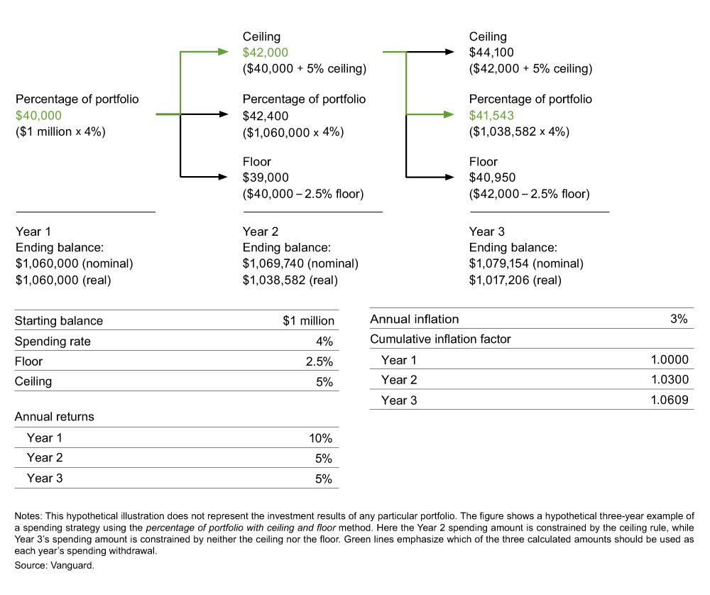
As previously mentioned, our dynamic spending rule is a hybrid of these two rules. With this rule, withdrawals are kept within a maximum percentage increase and minimum percentage decrease in real (inflation-adjusted) spending. The rule allows retirees to benefit from good markets by spending a portion of their gains, while weathering bad markets without a significant reduction in spending. Retirees accomplish this by saving some of their upside returns for use on a rainy day when the portfolio otherwise would have required a more significant reduction in spending (see the box below for an in-depth example of this spending rule).
To implement the dynamic spending rule, a retiree calculates each year’s spending by taking a stated percentage of the prior year-end’s real portfolio balance. The retiree then calculates a ceiling and a floor by applying chosen percentages to the previous year’s real spending amount, such as a 5% ceiling (increase) and a –2.5% floor (decrease). The results are then compared. If the newly calculated spending amount exceeds the ceiling, the spending amount will be limited to the ceiling amount; if the calculated spending falls below the floor, the spending amount is increased to the floor amount. With this rule, depending on the ceiling and floor selected, spending can therefore be made relatively consistent while remaining responsive to the financial markets’ performance—thereby helping to sustain the portfolio to meet future goals.
As Figure 1 illustrates, although the percentage of portfolio rule may have the highest rate of portfolio success and the highest internal rate of return (charts a and b), those come with a cost—namely, higher volatility in annual real spending (chart d). However, by implementing Vanguard’s hybrid approach, a retiree can capture many of the benefits of this approach while still significantly reducing the variation in annual spending that could occur as a result of market movements.
We examined the trade-offs mentioned previously in a multiplier framework [that is, a multiple of initial balance or spending amounts over 35 years for each spending rule (see charts c and d in Figure 1)]. For example, the dollar plus inflation rule produced real ending balances ranging from zero times the initial amount at the 5th percentile to 5.9 times the initial amount at the 95th percentile (chart c). In practical terms, this would correspond to an investor with a starting portfolio balance of $1 million and a 5% withdrawal rate ending with an account balance somewhere between $0 and $5.9 million 90% of the time. As chart c in Figure 1 shows, the two other approaches produced results in a much narrower range.
The most important trade-off when discussing a spending method, however, is spending volatility. Our analysis shows that, on average, the dollar plus inflation rule produces a real annual spending multiplier of 1.0, unless the portfolio depletes, in which case it falls to zero (see chart d in Figure 1). Continuing the example from the previous paragraph, in theory, this simply means real annual spending of $50,000 or $0. In reality, an investor would not let his or her portfolio drop to $0, but would potentially have to make uncomfortable adjustments along the way. The dollar plus inflation rule is thus strikingly insensitive to market conditions.
On the other hand, the percentage of portfolio rule produces real annual spending multipliers ranging from 0.4 to 2.0 at the 5th and 95th percentiles and 1.0 on average, while the dynamic spending rule’s multiples range from 0.5 to 1.8 at the 5th and 95th percentiles and also average 1.0. It bears repeating that, in this latter example using the dynamic spending approach, one’s real spending would never decrease by more than 2.5% or increase by more than 5% in any given year; use of the percentage of portfolio approach, however, could result in real spending decreasing or increasing by a theoretically unlimited amount (although, in reality, bounded by the portfolio’s performance and, hence, that of the financial markets). Ultimately, an investor with endless flexibility would likely choose the percentage of portfolio approach; however, for most retirees this is simply not practical. In that case, dynamic spending can provide many of the benefits of the percentage of portfolio rule without giving up the relatively consistent level of real annual spending.
An important point in this discussion is that the outcomes are significantly affected by the selection of the ceiling and floor percentages; this is where retirees, and their advisers, can tailor the ceiling and floor percentages along the spectrum (from a 0% ceiling and 0% floor to an unlimited ceiling and an unlimited floor) to provide the flexibility each retiree needs to meet his or her unique goals. For illustrative purposes, we used the 5% ceiling and the 2.5% floor as an initial starting point because it provided a portfolio survival rate of 85% over a 35-year time horizon; however, we tested hundreds of ceiling and floor scenarios to determine the impact on portfolios’ success rates.
Figure 2 highlights two scenarios. The first scenario (chart a) held the ceiling constant at 0%—meaning any excess returns were reinvested in the portfolio (as opposed to increasing the spending amount)—and tested the impact on portfolio success rates of different floor percentages in –0.5% increments between 0.0% and –12.0% (0.0%, –0.5%, –1.0%, –1.5% . . . –11.5%, –12.0%). The second scenario (chart b) held the floor constant at 0%—meaning spending could not decrease—and tested different ceiling percentages between 0.0% and 12.0% in 0.5% increments.
Figure 2. Dynamic Spending Floor and Ceiling Sensitivity
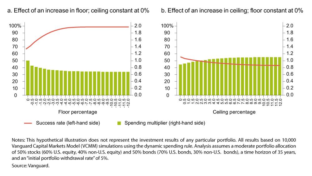
Our analysis found that the more flexibility retirees have in their floor—meaning, the more they are able to reduce spending when the markets are performing poorly—the higher their success rate, meaning the lower the chance that they will deplete their portfolio or be required to significantly reduce their spending before the end of their planning horizon. In fact, retirees’ ability to accept changes in their floor helps their portfolio more than increasing their ceiling hurts it. For example, a ceiling/floor combination of 0% and –1% is about 12 percentage points more successful, as measured by success rate, than a ceiling/floor combination of 0% and 0% (i.e., dollars plus inflation). On the other hand, a ceiling/floor combination of 1% and 0% is about four percentage points less successful than a ceiling/floor combination of 0% and 0%. This is shown in chart a of Figure 2, where the absolute slope of the line when keeping the ceiling constant (chart a) is much steeper than that of the line when keeping the floor constant (chart b).
This concept has implications for retiree withdrawal rates, as shown in Table 1. The table shows portfolio withdrawal rates for both a 0%/0% ceiling/floor rule and a 5.0%/–2.5% ceiling/floor rule using different time horizons and asset allocations assuming an 85% success rate. As the table shows, retirees who can incorporate flexibility into their annual spending needs are able to set higher initial portfolio withdrawal rates, which can help them be in a better position to meet their near-term financial goals. (We assume that a conservative asset allocation corresponds to a 20% stock/80% bond portfolio, a moderate asset allocation corresponds to a 50% stock/50% bond portfolio and an aggressive asset allocation corresponds to an 80% stock/20% bond portfolio.)
Table 1. Portfolio Initial Withdrawal Rates (%) for Various Asset Allocations and Time Horizons
For example, a moderate investor who wants stable inflation-adjusted spending (that is, a 0% ceiling and a 0% floor) with a 35-year time horizon can set an initial portfolio withdrawal rate of 3.9%, assuming an 85% chance that he or she will not run out of money. If that same retiree can cut spending back by 2.5% in years when the market is performing poorly, and if he or she can limit increases in annual spending to 5.0% in years when the markets are performing well, the retiree could set the initial portfolio withdrawal rate at 5.0%, which is 1.1 percentage points higher than the previous example.
In short, when choosing a floor and ceiling combination, there are trade-offs between maintaining the desired level of current spending (spending percentage) and preserving the portfolio to support future spending/goals (success rate). In selecting a floor and ceiling, retirees and their advisers must have a solid understanding of their income and expenses; the more they can tolerate some short-term fluctuations in spending, the more likely they are to achieve their longer-term goals.
Finally, once a spending strategy and a withdrawal amount have been selected, possible implementation strategies include:
The process for using the dynamic spending rule is:
In short, this rule helps retirees maintain income for basic expenses while allowing for more discretionary income if market returns are favorable.
Figure 3. Dynamic Spending Strategy Example: Percentage of Portfolio With Ceiling and Floor
Financial Planning

Financial Planning
Portfolio Strategies

Henry Hanau from NY posted over 9 years ago:
Doug from NY posted over 9 years ago:
Charles Rotblut from IL posted over 9 years ago:
Joseph Crowley from AZ posted over 9 years ago:
Donald Licatovich from TX posted over 9 years ago:
Andrew Shuman from ME posted over 9 years ago:
Ed Ehrhart from CA posted over 9 years ago:
Mike from CA posted over 9 years ago:
Adam Gallucci from MA posted over 9 years ago:
David Vigil from CO posted over 9 years ago:
Joe Weishaupt from PA posted over 9 years ago:
Gary Ryba from MN posted over 9 years ago:
Gary Ryba from MN posted over 9 years ago:
Joseph Dixon from VA posted over 9 years ago:
Charles Rotblut from IL posted over 9 years ago:
Mel Meyer from IL posted over 9 years ago:
Mitch from HI posted over 9 years ago:
Chris from California posted over 9 years ago:
Richard Shaw from AZ posted over 9 years ago:
Victor from NC posted over 9 years ago:
Doug from NY posted over 8 years ago:
Gregory Boger from FL posted over 8 years ago:
You need to log in as a registered AAII user before commenting.
Log InCreate an account