The father of value investing, Benjamin Graham, advised us when investing to buy stocks that have a margin of safety—that is, those that are priced at a discount to their intrinsic value. A stock’s intrinsic value is determined by making a calculation or using a financial model. Remember, if a stock’s price reflects its intrinsic value, it is unlikely to outperform the market. We need a way, therefore, to determine that value.

The value of any financial asset, including a stock, is the sum of its future cash flows, each discounted back to the present. Those cash flows can be earnings, free cash flow or even the future sale price we expect to receive when we ultimately sell the stock. For a stock that pays dividends, the dividend discount model allows us to calculate the present value of its future expected dividends, and therefore arrive at an estimate of its intrinsic value. However, it is impossible to know a stock’s “true” intrinsic value since the future is unknown. Our discussion, therefore, relates to making assumptions about future dividends to value a stock. There are other methods than can be used, which can arrive at different estimated values.

Dividend Discount Model

The dividend discount model uses several inputs: the most recent dividend and the rate at which we expect future dividends to grow expressed as a percentage. These are expected future dividends, but since money in the future is (usually) worth less than money today, we need to calculate their present value using a discount rate. This rate is often referred to as the cost of equity, although I prefer to use the term risk-adjusted discount rate.

The model can be written as a formula illustrating that the stock’s present value is the sum of its future dividends, which we can denote as D₁, D₂, each representing a year, out to infinity, each discounted back to the present:

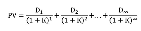
If we assume that dividends grow at a constant rate, we can use a simplified version, known as the constant growth, or Gordon growth, model:

PV = [D₀ (KO) (1 + g)] ÷ (K – g)

Where:

• PV = present value of the stock
• D₀ = last year’s dividend
• g = dividend growth rate
• K = discount rate

Since next year’s dividend is assumed to have increased from last year’s at the dividend growth rate, we can also write the formula as:

PV = D₁ ÷ (K – g)

We can obtain the firm’s dividend history from sources such as Yahoo Finance and use that to determine their historical growth rate. [AAII members can find any stock’s five-year dividend growth rate using the search tool on AAII.com; at the Stock Evaluator page, scroll down to the growth section of the financial summary.]

Now, we have to determine the appropriate discount rate to use.

Discount Rate

When setting a discount rate, it’s helpful to understand how bank lending is, in some regard, similar to insurance. A car insurance firm collects premiums from its customers and, in turn, promises to pay them if their cars become damaged or they injure others. The insurer typically uses risk-based pricing, where larger premiums are charged to customers considered to be riskier. In aggregate, the insurer expects that premiums collected will be sufficient to provide the firm with a profit once it has paid any claims submitted.

Similarly, banks set the interest rates they charge on loans by charging higher rates to their riskier borrowers. They expect some borrowers to default, but hope that the interest received, combined with reserves, will be sufficient to cover defaults and generate a profit.

Discount rates for investment purposes can be viewed in the same way. Imagine two borrowers, Jack and Jill, who wish to borrow $100 from us for one year. We consider Jack to be low risk, and so charge him an interest rate of 5%, while we charge Jill, whom we view as high risk, 10%. Assuming neither borrower defaults, in a year’s time Jack will pay us $105 and Jill will pay $110.

Since we’re willing to lend to Jack, we can argue that, ignoring any profit motive, we’re indifferent between having $100 today and receiving his $105 in the future. Using this logic, Jack’s expected future repayment of $105 is worth $100 today [$105 ÷ (1 + 0.05)], with 5% representing the appropriate discount rate. Similarly, Jill’s expected future repayment of $110 is worth $100 today [$110 ÷ (1 + 0.10)], with 10% being the discount rate appropriate when viewing Jill’s obligation. The present value of a sum of money to be received in the future depends on the discount rate, which is a function of how the lender or investor perceives risk (the likelihood of not receiving the money). We consider the appropriate discount rate for Jack’s loan repayment to be 5%, while the discount rate for Jill is 10%. Jill’s rate is higher because it is adjusted for her specific risk. We can refer to the rates of 5% and 10% as the risk-adjusted discounted rates for Jack and Jill, respectively.

Risk-Adjusted Discount Rate

When calculating the present value of a firm’s future dividends, we use a discount rate appropriate for the firm’s level of risk, as we perceive it. A common approach, based on a theoretical financial model known as the capital asset pricing model (CAPM), is to use a risk-free rate, usually the yield on a 10-year Treasury note, plus an equity risk premium equal to the firm’s beta multiplied by the market risk premium. The risk-adjusted discount rate formula is, therefore:

K = RF + (B (KO) MRP)

Where:

• K = risk-adjusted discount rate
• RF = risk-free rate
• B = beta
• MRP = market risk premium

Beta is a measure of a stock’s risk relative to the market, usually the S&P 500 index. The market’s beta is always 1.00; a beta higher than 1.00 indicates that, on average, when the market rises, the stock will rise to a greater extent and when the market falls, the stock will fall to a greater extent. A beta lower than 1.00 indicates that, on average, the stock will move to a lesser extent than the market. The higher the beta, the greater the risk.

One problem with this approach is that beta, one of several measures of a firm’s riskiness, changes depending on when and how you calculate it. Another issue is that we don’t know exactly what the market risk premium is. Reflecting the extra return that investors require to be in the stock market over the bond market, it is generally in the range of 4% to 6%. The stock market is generally perceived to be risker than the bond market because of the uncertainty of receiving cash flows. Estimates may vary depending on market and economic conditions.

I should note that, although popular in textbooks, many well-known investors don’t agree with this method of determining discount rates. They prefer to use a base rate (for example, 10%) for all firms they consider to have average risk, increasing it (perhaps to 12%) for more risky firms and decreasing it (to perhaps 8%) for less risky firms. Warren Buffett is reported to simply use the yield on the 10-year Treasury bond, while accounting for risk by being conservative in the growth assumptions he makes. In this article, however, the CAPM approach is used.

Example Using Coca-Cola

At the time of writing (October 3, 2023), Yahoo Finance reported that the price of Coca-Cola Co. (KO) stock was $54.80 per share, its beta was 0.55 and the 10-year Treasury yield (risk-free rate) was 4.78%. For the market risk premium, I use the projections of Aswath Damodaran, a corporate finance and valuation professor for the Stern School of Business at New York University. Per these projections, the market risk premium was shown as 4.47%. The risk-adjusted discount rate for Coca-Cola stock is therefore:

= RF + (B (KO) MRP)
= 4.78% + (0.55 (KO) 4.47%)
= 7.24%

The historical data tab on the Yahoo Finance page for Coca-Cola shows us that the dividend over the last year totaled $1.82 per share (0.46 + 0.46 + 0.46 + 0.44). We can also see that five years ago it was $1.56, so we can estimate the annual dividend growth rate as:

= (1.82 ÷ 1.54)^(1/5) – 1
= 3.4%

[AAII members would currently see 3.6% for Coca-Cola’s five-year dividend growth rate at the stock’s evaluator page due to different time periods used in the calculation.]

Plugging these assumptions into the Gordon growth model, we calculate a value of $49.01:

= [D₀ (KO) (1 + g)] ÷ (K – g)
= [1.82 (KO) (1 + 0.034)] ÷ (0.0724 – 0.034)
= 1.88188 ÷ 0.0384
= $49.01

The model’s value, $49.01, was less than the stock’s market price of $54.80. However, if we were to increase the assumed growth rate in dividends from 3.4% to 3.8%, the model valuation would be $54.92, very close to the $54.80 market price. Given that Coca-Cola’s annual dividend has increased by 5.4% recently, assuming dividends will grow at 3.8% annually in the future might be justified, which suggests that the stock is reasonably priced—at least when considered in the context of dividends.

Stocks With High Growth Rates

While the Gordon growth model seems to work well for Coca-Cola, what about for a firm that has a relatively high dividend growth rate? Let’s look at Microsoft Corp. (MSFT).

According to Yahoo Finance, Microsoft’s beta was 0.90, its stock price was $314.00, its most recent dividend was $2.72 and the average annual dividend growth rate for the last five years was 10.12% [10.0% at Microsoft’s evaluator page on AAII.com]. Using the risk-free rate and market risk premium from our Coca-Cola example, we get a risk-adjusted discount rate of:

= RF + (B (KO) MRP)
= 4.78% + (0.90 (KO) 4.47%)
= 8.8%

Applying these inputs to our model produces a present value of –$226.90.

= [D₀ (KO) (1 + g)] ÷ (K – g)
= [2.72 (KO) (1 + 0.1012%)] ÷ (0.088 – 0.1012)
= 2.9952 ÷ –0.0132
= –$226.90

In this case, the model breaks down, returning a negative price. This example illustrates two problems with the Gordon growth model. The first is mathematical, arising from the fact that the assumed dividend growth rate of 10.12% exceeds the discount rate of 8.8%, so that the denominator is negative, leading to a negative estimate of the stock’s value. A second issue relates to the reasonableness of the growth assumption. While it might be reasonable to assume that Microsoft could continue to increase dividends at a rate of 10% for the foreseeable future, it is not plausible that Microsoft’s dividends could grow at a faster rate than the U.S. gross domestic product (GDP) forever. Since GDP is expected to grow at around 4% annually (2% real and 2% inflation), our model should use a dividend growth rate that does not exceed 4% in the long run.

Two-Stage Dividend Discount Model

One solution to the problems caused by high growth rate assumptions is to break the future life of the firm into two periods, or stages. In the first, high-growth, stage, which we’ll assume extends for 10 years, we will allow the dividends to grow at a high rate. For our Microsoft example, I use the 10.12% recent growth rate, so that the dividend grows from last year’s $2.72 to $7.132 in year 10.

= 2.72 (KO) (1.1012)¹⁰
= $7.132

For the second stage, we now imagine that we’ve jumped 10 years into the future to 2033. If we were to value the stock at that time, using a plausible long-term growth rate assumption of 3.5%, and the dividend of $7.132 that we expect to be paid in 2033, we would arrive at a stock value of $139.28:

= [D₁₀ (KO) (1 + g)] ÷ (K – g)
= [7.132 (KO) (1 + 0.035)] ÷ (0.088 – 0.035)
= 7.38162 ÷ 0.053
= $139.28

This result of $139.28 reflects the value, in year 10, of all dividends from year 11 into the future and is referred to as the terminal value. You can consider it to be the price at which we could sell the stock, in year 10, to someone valuing the firm using the Gordon growth model at that time.

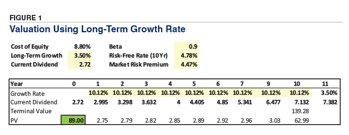
To calculate the value of the firm today, in 2023, we need to account for the value of the dividends to be received in years 1 through 10, and we need to discount the terminal value of $139.28 back to the present, as illustrated in Figure 1.

Per Figure 1, the year 10 cash flow includes the assumed dividend of $7.132, plus the terminal value of $139.28, reflecting all subsequent dividends. Since these cash flows are in year 10, we need to discount them back to the present:

= (7.132 + 139.28) ÷ (1 + 0.088)¹⁰
= $62.99

In a similar fashion, we discount the cash flows for years 1 through 9, in which we only receive dividends, back to the present. The sum of the present values, reflecting the value we estimate for the firm, is $89.00. However, since Microsoft is currently trading at a price of $314.00, there seems to be a large disconnect between our valuation and the market price.

Adjusting the Terminal Value

A firm such as Microsoft that has been growing rapidly clearly presents problems when using the dividend discount model. One solution is to assume that the period of high growth extends out longer than 10 years. In reality, and given our other assumptions, the period of high growth would have to extend out 55 years to justify the current price of $314.00. We can combine the formula for the present value of a growing annuity with the Gordon growth model to produce a general formula for a two-stage model:

Where:

• L = long-term growth rate
• n = duration of high-growth stage

Plugging in same the values for Microsoft in our example, but assuming that the duration of the high-growth stage is 55 years, and the long-term dividend growth rate is 3.5%, we can calculate the value as:

= (–226.91 (KO) –0.9411) + (565.133 ÷ 5.481)
= 213.55 + 103.1063
= $316.66

Calculating Terminal Value Using the Price-Earnings Ratio

The Gordon growth model can, using reasonable assumptions, determine a value for a low-growth stock such as Coca-Cola as shown in our first example. On the other hand, to produce a value for a high-growth stock such as Microsoft, we must assume that the high rate of dividend growth will continue for a prolonged period. In our example, this is 55 years.

An alternative approach that doesn’t require us to make assumptions about growth rates for an extended period is to calculate the terminal value using a price-earnings (P/E) multiple. Rather than using the Gordon growth model to calculate the terminal value, which you will recall reflects an estimate of the price that someone would pay for the firm in the future, we can instead calculate the terminal value as earnings per share (EPS) multiplied by the price-earnings ratio.

Returning to our Microsoft example, we need two additional pieces of information, the earnings per share and the price-earnings ratio, both of which we can obtain from Yahoo Finance [and from the financial summary on the stock’s evaluator page at AAII.com]. Microsoft’s most recent earnings as shown at Yahoo Finance were $9.69 per share, and the price-earnings multiple was 32.0. Since the most recent annual dividend was $2.72, we can calculate the dividend payout ratio as:

= Dividend ÷ EPS
= 2.72 ÷ 9.69
= 28.07%

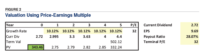
Figure 2 shows a revised model that projects dividends growing at 10.12% for five years to reach $4.404.

= 2.72 (KO) (1 + 0.1012)⁵
= $4.404

If we assume that Microsoft continues to pay 28.07% of earnings in the form of dividends, then we can say that the year 5 dividend of $4.404 represents 28.07% of the firm’s earnings that year, which must therefore equal $15.69:

= 4.404 ÷ 0.2807
= $15.69

If investors are willing to pay a price-earnings ratio of 32.0 for Microsoft in five years, then the sale price will be $502.12:

= $15.69 (KO) 32.0
= $502.12 (rounded)

This sale price, which is our terminal value, needs to be discounted back to the present along with the annual dividends in each of the five years, resulting in a current valuation of $343.46.

Given the assumptions we have made—that dividends will continue to grow at a rate of 10.12% for five years and represent 28.07% of earnings, that the risk-adjusted discount rate of 8.8% is appropriate and that investors will be willing to pay a price-earnings multiple of 32.0 in five years—then Microsoft’s stock, which we value at $343.46, looks to be slightly underpriced in the market at $314.00.

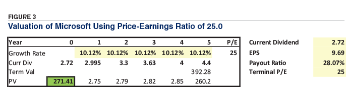
However, if we believe that dividends will indeed grow at 10.12%, but that investors in five years will pay a lower price-earnings multiple of, say, 25.0, then our estimated value for Microsoft will be $271.41 (see Figure 3). We can see that the value produced by the model depends on the price-earnings multiple that is assumed.

Conclusion

The dividend discount model offers an intuitive method to value a stock. It can be instructive for both low-growth and high-growth stocks, although the latter will require us to use a two-stage model rather than the one-stage Gordon growth model. Both forms of the model can allow us to explore the assumptions that are currently priced into the stock by the market and to decide for ourselves if we believe those assumptions are justified or not.

While the dividend discount model only applies to stocks that pay dividends, it is similar in form to other discounted cash flow models that use free cash flow or other inputs.

The value produced by the model is a function of the discount rate used, the growth rates assumed and the terminal value. If you are optimistic about the prospects of a stock, you can use the model to calculate price targets.

It should be stressed that this model makes assumptions about management’s commitment to continue paying a dividend and, when using a price-earnings multiple to calculate the terminal value, assumptions about the payout ratio and the multiple that investors are willing to pay in the future. As with all other models, investors should exercise caution! 

Related

Investor Professor

Three Pillars for Successful Dividend Investing

Related

Stock Strategies

Methods for Valuing a Stock Based on Profitability and Growth

Related

Stock Strategies

Valuing Young Growth Companies