An investor who purchased a 10-year Apple bond, with a coupon (annual interest) of 2.4% when it was issued in 2013, would have seen the value of his investment drop 12% over the following four months.

Meanwhile, if he owned long-maturity U.S. Treasury bonds because they were “risk-free,” he would probably have been pleasantly surprised to learn that in 2014 they returned 25%. How, he might ask, can this be? Isn’t the fixed-income market supposed to be the “safe” asset class? How can high-quality bonds like those issued by Apple or the U.S. Treasury, with yields in the low single digits, exhibit levels of price volatility that might normally be associated with the stock market?

In order to answer these questions, we need to understand how bonds are affected by changes in interest rates.

Change in Yield

The yield (income return) on a Treasury bond can change for a variety of reasons, such as actions by the Federal Reserve, a change in economic conditions, and supply and demand. Corporate bonds can also be affected by changes in the perceived risk of the issuer or sector. Such changes in yield will cause a bond’s price to move.

Let us imagine that an investor, Joe, owns a 10-year bond with a 10% coupon paid semiannually and a principal amount of $1,000. He will receive $50 in interest every six months, plus the $1,000 principal on the maturity date in 10 years. If market yield for other 10-year bonds with the equivalent risk profile is also 10%, then Joe’s bond will be priced at par, which is $1,000.

Now imagine that yields for these bonds increase by one percentage point (100 basis points) to 11% as soon as Joe made his purchase. Joe’s bond will immediately drop in price.

We can use several different approaches to explain why. First, as I explained in “Bond Pricing Made Simple” (November 2015 AAII Journal), the price of a bond is the present value, at the prevailing yield, of its expected future cash flows. Because the yield has increased to 11%, Joe must now discount each payment, including the principal to be paid at maturity, at this higher discount rate. The bond’s price will therefore drop.

Formula 1 (shown in the accompanying box below), which some of you may recognize from my previous article, calculates the value of a bullet bond with periodic interest payments from my November 2015 article. (The term “bullet bond” refers to a bond whose principal can solely be paid at maturity.) When used to determine the value of Joe’s bond, the formula’s calculation is:

Alternatively, we could explain that, because the market is now offering bonds with a yield of 11%, Joe’s bond with its yield of 10% is no longer attractive. His bond must, therefore, drop in price to appeal to other investors; this will increase the yield, or return, that a purchaser would obtain. The coupon is still 10%, but the yield increases to 11%. If the price drops below $1,000 to $940.25 then a buyer’s return would increase, since he would receive not only the coupon return ($50 every six months), but also a capital gain equal to the difference between the price that he pays, $940.25, and the $1,000 principal that he will receive at maturity. The capital gain combines with the coupon return to result in a yield of 11%, precisely what the market demands.

Relative Coupon Method

While bond textbooks will offer the two preceding explanations, I have an alternative explanation that I believe makes more intuitive sense. I call it the Relative Coupon approach. Let’s use it to consider Joe’s situation. If he holds the 10% coupon bond in an 11% world, he is at a disadvantage because he receives only $100 a year in coupon payments, whereas an 11% bond would pay him $110 per year. He therefore suffers a shortfall of $10 each year (or, more precisely, $5 every six months) for 10 years. We can easily determine the value of this shortfall by using a long and short perpetuity, as in Formula 2 in the box below.

In this case, the periodic cash flow shortfall is the difference between the $55 coupon paid every six months on a par bond and the $50 coupon paid on Joe’s bond every six months. The math, using Formula 2, is:

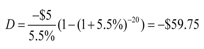
Using this Relative Coupon approach, we see a discount to par of $59.75. So the bond’s price is $1,000 – $59.75, or $940.25, just as we calculated using Formula 1. Note that in Formula 2 we are valuing not the coupon payment, but rather the stream of cash flow differences that arise when our bond pays a coupon different to that on the par bond—that is, the market yield. (We can ignore the principal due at maturity since it is the same in both cases.)

Now suppose yields, instead of increasing to 11%, were to drop to 9%. Joe, with his 10% bond, would now be better off, relative to holding a new 9% bond, to the tune of $10 per year ($5 every six months) for the 10-year life of his bond. Instead of a periodic shortfall, he now benefits each month. The present value of this stream of cash flow differences, again using Formula 2, is:

Instead of being priced at a discount, the bond is priced at a premium of $65.04. By holding the 10% bond Joe is better off, relative to the holder of a 9% $1,000 par bond, by $65.04. His bond is therefore worth $1,000 + $65.04, or $1,065.04.

Convex Price/Yield Relationship

Note that the amount that Joe would gain if the yield drops to 9% is more than he would lose if the yield increases to 11% ($65.04 versus $59.75), even though in both cases the gain or loss is simply the present value of the same stream of $5 cash flow differences. This asymmetry exists because we are valuing the two cash flow streams at different discount rates (the rate of return used to calculate the present value of a stream of future cash flows); the lower the discount rate, the higher the present value.

Figure 1. Price of 10-Year 10% Coupon Bond

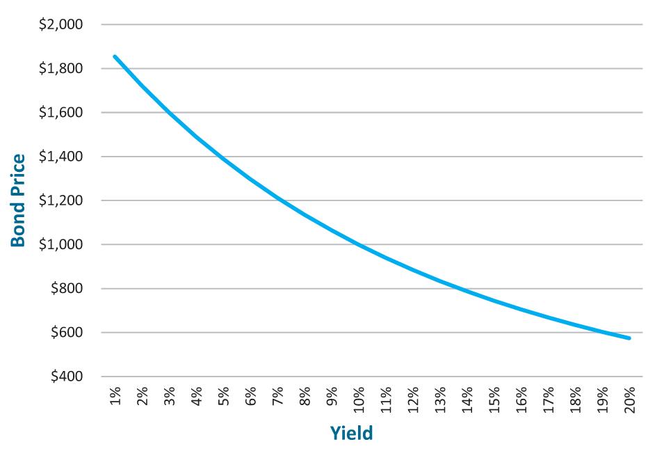
In fact, we can use this Relative Coupon approach to quickly calculate the bond price at yields ranging from, say, 1% to 20%. Figure 1 illustrates how prices don’t change linearly with changes in yield but in a curved fashion. As yields decrease, prices increase rapidly (gaining $854, for example, if the yield drops 9% from 10% down to 1%), whereas when yields increase, prices decrease at a slower pace (a yield increase of 9% to 19% results in a price of $603, a drop of only $397). This asymmetry results in the price/yield curve being convex (bulging out, as opposed to being a straight diagonal). So we refer to a typical bond as having positive convexity. (While it is beyond the scope of this article, callable bonds and mortgage-backed securities can exhibit negative convexity.)

Modified Duration

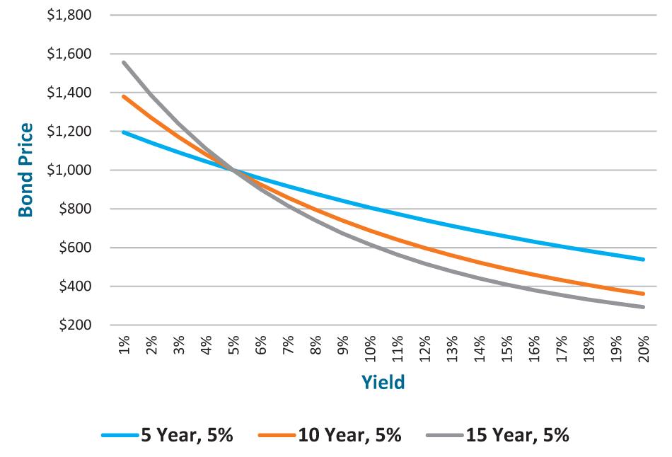
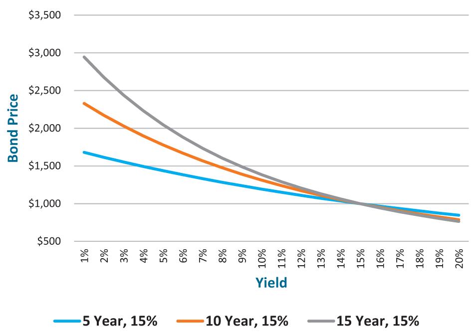
Bonds don’t all respond exactly the same to a given interest rate change. Some will be more price-sensitive, and others less, than Joe’s bond. Figures 2 and 3 show prices for five-, 10- and 15-year bonds at yields ranging from 1% to 20%. In Figure 2 you can see that the prices of 5% coupon bonds range from about $300 to about $1,600, while in Figure 3 you can see that 15% coupon bonds range in price from about $800 to about $3,000, depending on yield and maturity. It appears that bond prices can exhibit significant volatility, depending on yield movements.

Figure 2. Price/Yield for 5% Bonds

Figure 3. Price/Yield for 15% Bonds

Because the impact of a given change in yield depends on a bond’s coupon, maturity and yield, and because it traditionally has been cumbersome to predict, bond investors often use an approximation known as a bond’s modified duration. For small changes in yield, a bond’s percentage price change can be approximated with Formula 3 in the box below.

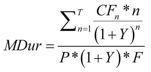
The modified duration measure is the weighted average time to the receipt of a bond’s cash flows, on a present value basis, divided by one plus the periodic yield as shown in Formula 4 in the box below.

The modified duration for Joe’s 10% coupon bond at a yield of 10% is 6.23. (The Excel MDuration() formula produces the same result as Formula 4). Using Formula 3, we can approximate the price change for a given yield change. For example, if the yield increased 1%, from 10% to 11%, then the approximate price change is:

So a 1% increase in yield changes the price by 6.23% from $1,000 to about $937.70. This is close to the actual price of $940.25 that we calculated for Joe’s bond at an 11% yield.

While the modified approximation is close, although not exact, for small rate changes, as the yield change increases the predicted price move becomes less and less accurate. For example, at a yield of 20%, which is a 10-percentage-point increase, the change in price calculated by Formula 3 is:

Such a move would cause the price to drop $623, from $1,000 to $377. However, we can calculate the correct decline using Formula 2:

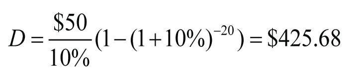
The price decline in reality will be $425.68, so the bond’s price would be $574.32, almost $200 higher than was predicted by the modified duration approximation. This significant error in prices predicted using modified duration arises from the nonlinear, or convex, nature of the price/yield curve. To improve their estimates of price changes, professional investors use an adjustment to modified duration, called the convexity measure. While that refinement reduces the error in price approximations, it does not eliminate it.

Precisely Predicting Price Moves

With the tools now in our toolbox there is no need for us to resort to the crude approximations calculated using modified duration. Instead, we can use Formula 1 to directly calculate the price at a given yield, using the Sum of Perpetuities method introduced in my November 2015 AAII Journal article. Alternatively, we can use the Relative Coupon method and extend Formula 2 to measure the change in a bond’s premium or discount as shown in Formula 5 in the box below.

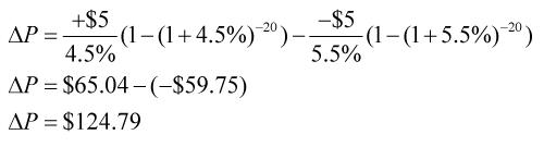
Let’s suppose Joe’s bond is trading at 11%, and we want to see what happens if the yield were to move to 9%. The periodic cash difference at 11% is (10% – 11%) × $1,000 ÷ 2, or –$5. At 9% the periodic cash difference is +$5. Plugging the appropriate values into Formula 5, we have S1 equal to 9% ÷ 2 and S0 equal to 11% ÷ 2, as shown in Example A.

Examples of Calculating Changes in Bond Prices

Example A

Example B

Example C

Joe’s 11% bond, which we know is trading at a price of $940.25, will therefore respond to a 2% decrease in rates (11% down to 9%) with a price increase of $124.79. The new price will be $940.25 + $124.79 = $1,065.04, matching our earlier calculation. To mirror modified duration, we can divide the price change by the price to see the percentage price move.

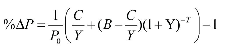
Alternatively, we can extend Formula 1 to determine the percentage price change at a new yield, shown in Formula 6.

Caveat

Investors need no longer accept the inaccuracy of modified duration and convexity when, using the formulas introduced here, it is easy to calculate with precision the price corresponding to a given yield.

We should note, however, that these formulas apply only to non-amortizing bonds and not, for example, to mortgage-backed securities.

Apple and Treasury Bonds

So what happened to Treasury bonds in 2014? Yields dropped from 3.97% at the start of the year to 2.73%. Assuming that a 30-year Treasury bond was priced at par (and therefore had a coupon of 3.97%, paying $19.85 every six months) on December 31, 2013, one year later it would be a 29-year bond with a yield of 2.73%. Plugging into Formula 1 would result in a 25% gain over its $1,000 starting value, as shown in Example B.

As for the Apple bond, it was issued in April 2013 at a yield of 2.4%, and yields increased to 3.92% in September 2013. Using Formula 6 this time, and allowing for one six-month period that has elapsed, we get a decline of about 12%, as shown in Example C.

Summary

Bond investors, even those who purchase U.S. Treasuries and highly rated corporate bonds, need to be aware of a bond’s price sensitivity to changes in interest rates, which can result from changes in Federal Reserve policy, market optimism, liquidity demands, corporate risk and other factors.

Interest rate sensitivity traditionally is estimated using a bond’s modified duration, but for regular bonds can be determined precisely using the Sum of Perpetuities and the Relative Coupon methods illustrated here.

Bond Formulas

Formula 1

The price of a bullet bond with periodic interest payments can be calculated by using the values of the perpetuities and the principal bullet:

 

 

 

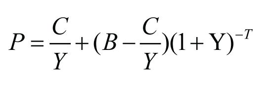
Where,

• P is the bond price,
• C is the periodic coupon payment,
• Y is the periodic yield,
• B is the principal bullet at maturity, and
• T is the number of periods to maturity.

Note that the valuation expression for a perpetuity will be undefined at a yield equal to zero. When the yield to maturity is zero, the price of a bond is simply the undiscounted sum of all coupon and principal cash flows. However, in practice the formula can be used if an infinitesimally small yield is assumed, such as 0.00001%.

Formula 2

The value of the difference in cash from holding a bond with an interest rate below or above the current market yield can be determined by using a long and short perpetuity:

 

 

Where,

• D is the premium or discount—that is, difference in value from a par bond,
• Y is the periodic yield,
• T is the number of periods to maturity, and
• S is the periodic cash flow shortfall (or increase)—that is, the difference between the coupon paid on a par bond and a bond with a lower (or higher) interest rate.

Formula 3

The percentage price change in a bond in response to small yield changes can be approximated with:

 

 

Where,

• %ΔP is the percentage change in price,
• ≈ denotes approximate change,
• MDur is the bond’s modified duration, and
• ΔY is the change in yield.

Formula 4

Modified duration measures the sensitivity of a bond’s price to interest rate movements. It is the weighted average time to the receipt of a bond’s cash flows, on a present value basis, divided by one plus the periodic yield:

 

 

 

 

Where,

• MDur is modified duration,
• CF_n is the cash flow at time n,
• Y is the periodic yield,
• P is the bond’s price and
• F is the frequency of payments, which is 2 for a typical semiannual pay bond.

Formula 5

The Relative Coupon method extends Formula 2 to measure the change in a bond’s premium or discount.

 

 

Where,

• ΔP is the change in price,
• S₁ is the periodic cash flow difference at the new yield,
• Y₁ is the new periodic yield,
• T the number of periods to maturity, and
• S₀ is the cash flow difference at Y_o, the current yield.

Formula 6

This extends Formula 1 to determine the percentage price change at a new yield.

 

 

Where,

• P₀ is the old price,
• C is the periodic coupon payment,
• Y is the new periodic yield,
• B is the principal bullet at maturity, and
• T is the number of periods to maturity.

Related

Bonds

Bond Pricing Made Simple

Related

Bonds

How Safe Are Municipal Bonds?

Related

Investor Professor

How Interest Rate Changes Affect the Price of Bonds