


"Annual income twenty pounds, annual expenditure nineteen nineteen and six, result happiness. Annual income twenty pounds, annual expenditure twenty pounds ought and six, result misery." —Mr. Micawber (From Charles Dickens’ “David Copperfield,” 1850)
Financing a safe retirement with a risky portfolio depends on trade-offs. Increasing spending today is desirable, but it increases the risk of shortfall in the future. High variation in spending is undesirable, but upward adjustments let you increase spending when investments outperform, while downward adjustments after underperformance reduce risk of even deeper future cutbacks. Finally, accepting future spending variation enables higher spending today, if you invest in higher-risk, higher-return portfolios, or accept a thinner buffer against downward adjustments.
William P. Bengen (1994) pioneered safe withdrawal literature by studying a constant spending strategy. Using this strategy, the retiree determines an appropriate spending amount at retirement, and adjusts it annually for inflation to achieve constant real spending. The model I discuss in this article is a generalization of the Bengen approach to incorporate a variable spending term (a fraction of a smoothed portfolio value, adjusted for remaining life expectancy). If you recalculate a Bengen rule and update spending every few years, or after significant portfolio changes, you approach a smoothed variable spending strategy. Everything that follows will use real, inflation-adjusted values.
In this article, I try to accomplish three things:
- Use Bengen’s approach to test strategies incorporating a constant and variable spending amount based on the size of the portfolio.
- Describe the shape of the trade-off: How much do shortfall risk and severity increase when you increase initial spending?
- Use certainty-equivalent spending to describe how, as you reduce your risk aversion and accept risk and variation in spending, you increase your lifetime spending.
The Withdrawal Rate Model
Bengen’s model had one parameter: constant spending. I added three parameters to determine variable spending that changes based on portfolio size:
- A smoothing parameter (n): I smooth spending variation by basing spending on an exponential moving average of the portfolio value.
- A mortality insensitivity parameter (b): I set the amount available to spend as the smoothed portfolio divided by the remaining life expectancy + b. An 80-year-old can safely spend a higher percentage of a $1 million portfolio than a 65-year-old, and higher b means spending adjusts more slowly as you age.
- A variable spending parameter (h): How much of the available amount is spent.
The complete spending model is:
si = K + EMA(P,n)i h
(Li + b)
Where (in addition to parameters above):
- si is spending in period I,
- K is constant spending,
- EMA(P,n)i is the exponential moving average of portfolio values and
- Li is the retiree’s remaining life expectancy in period i.
If h (variable spending) is 0, this reduces to the Bengen constant spending model. If K (constant spending) is 0, n is 1 (no smoothing) and b is large (minimal mortality updating), it’s similar to a constant percentage model that spends a fixed percentage each year.
Testing Variable Spending in Retirement
I tested about 3.7 million combinations of parameters and portfolios. The test subject is a hypothetical single 65-year-old male retiree, who chooses a withdrawal strategy and allocates between a U.S. large-capitalization stock index and a bond index. (The returns are represented by the Ibbotson data for large-cap stocks and intermediate-term U.S. government bonds from 1926–2012. For life expectancies, I used Social Security Administration actuarial life tables, which are at www.ssa.gov/oact/STATS/table4c6.html, accessed in May 2013.)
For each portfolio and set of parameters tested, I determined:
- Initial spending;
- Lifetime expected spending;
- Worst shortfall, defined as maximum decline below initial spending (I also calculated shortfall percentiles: 90th percentile = an outcome where 90% of outcomes had better worst-case shortfalls); and
- Shortfall probabilities (probability of a decline below initial spending; probability of 10% decline, etc.).
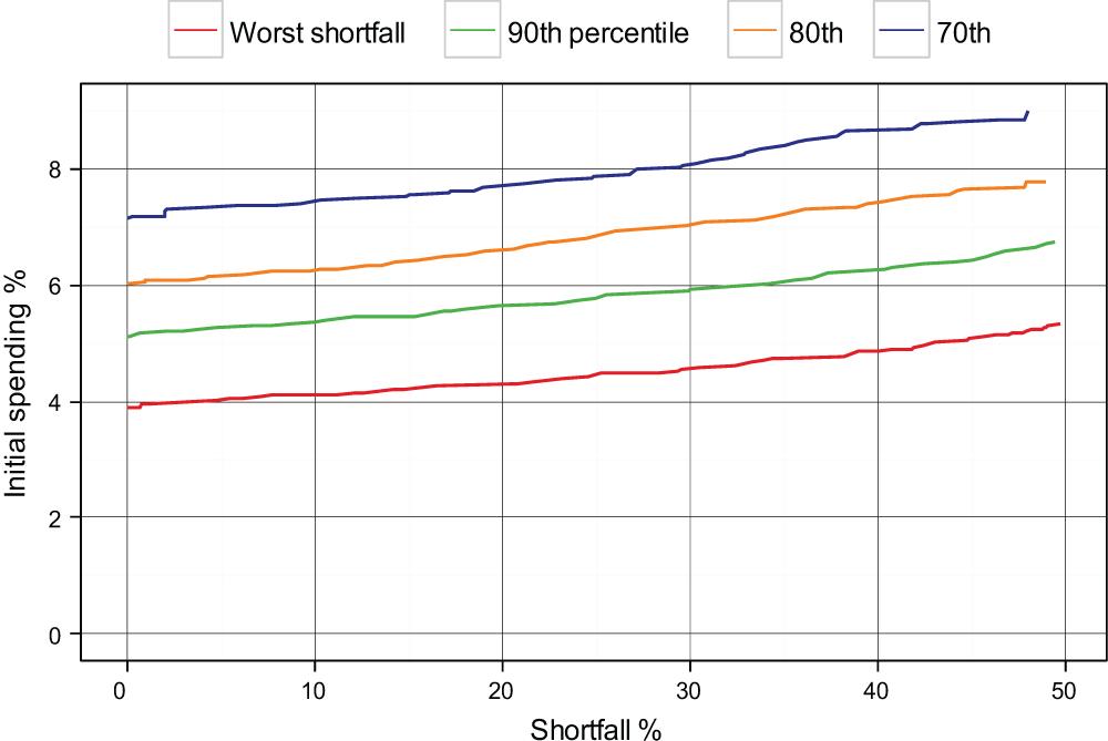
If a scatter graph with every possible combination of initial spending versus shortfall severity using every parameter value tested is plotted, a cloud is plotted. The top left boundary of the cloud represents the highest initial spending achievable for a given maximum shortfall. Figure 1 shows selected outcomes from this “possibility frontier” or “shortfall severity frontier.”
| Probability | ||||||||
| Initial | Worst | Equity | of 10% | Lifetime | ||||
| Spending* | Shortfall | Allocation | Constant | Variable | Mortality | Shortfall | Spending | |
| (%) | (%) | (%) | Spending | Spending | Smoothing | Insensitivity | (%) | (%) |
| 3.9 | 0.0 | 50 | 3.50 | 0.1 | 25.0 | 9 | 0 | 70.68 |
| 4.0 | 1.1 | 45 | 3.75 | 0.1 | 25.0 | 30 | 0 | 69.99 |
| 4.1 | 6.1 | 45 | 3.75 | 0.1 | 3.0 | 16 | 0 | 72.46 |
| 4.2 | 14.1 | 45 | 3.5 | 0.4 | 3.5 | 40 | 3 | 75.18 |
| 4.3 | 16.4 | 45 | 3.5 | 0.4 | 1.5 | 35 | 7 | 76.56 |
| 4.4 | 23.2 | 45 | 3.25 | 0.6 | 2.5 | 35 | 22 | 79.36 |
| 4.5 | 25.2 | 45 | 3.25 | 0.7 | 1.5 | 40 | 27 | 80.22 |
| 4.6 | 30.4 | 50 | 3.00 | 0.9 | 1.5 | 40 | 32 | 83.2 |
| 4.7 | 33.2 | 50 | 3.00 | 0.7 | 1.0 | 25 | 36 | 85.74 |
| 4.8 | 38.2 | 60 | 2.50 | 1.3 | 1.0 | 40 | 47 | 90.08 |
| 4.9 | 39.4 | 50 | 2.75 | 1.1 | 1.0 | 35 | 47 | 87.78 |
| 5.0 | 43.1 | 50 | 2.75 | 1.3 | 1.0 | 40 | 51 | 89.44 |
| 5.1 | 44.7 | 60 | 1.50 | 1.5 | 1.0 | 25 | 56 | 97.34 |
| 5.2 | 47.1 | 70 | 1.25 | 1.3 | 1.0 | 16 | 54 | 107.19 |
| 5.3 | 48.9 | 65 | 1.25 | 1.9 | 1.5 | 30 | 55 | 101.57 |
| 5.4 | 51.6 | 70 | 1.75 | 1.7 | 1.0 | 30 | 56 | 104.08 |
|
*The highest initial spending for a given maximum shortfall.
|
||||||||
The red line at the bottom (worst case) intersects the vertical axis at 3.9%, representing a strategy allowing 3.9% initial spending with worst-case decline from initial spending = 0% (no shortfall). The green line second from the bottom (90th percentile) intersects at 5.1%, indicating a strategy with 5.1% initial spending, which has no shortfall in 90% of outcomes. Observing where the 5.1% initial spending level intersects the red line, there is a strategy allowing 5.1% initial spending, which experienced a worst-case decline below initial spending of about 45%.
Minimum shortfall, maximum initial spending (bottom left) portfolios are highly diversified, with an emphasis on constant spending (high K) and little volatility in spending (low h). This closely matches the Bengen 4% solution. I found 3.9% to be the highest no-shortfall initial spending rate with a 50% equity allocation. (The difference is due to a methodological quirk: I withdraw each year’s spending from the portfolio at the beginning of the year, while Bengen withdraws at the end of each year. Using Bengen’s methodology, the retiree must prefund the first year of retirement, and 30 years of performance are considered for a 30-year retirement. Under my methodology, the retiree makes a withdrawal at the beginning of the first retirement year and each year thereafter through year 30, whose year-end performance doesn’t affect a withdrawal, hence 29 years of performance are considered. Bengen’s 4% could be viewed as my 3.9% of [retirement portfolio + prefunded first year]).
As initial spending is increased, the best achievable worst-case shortfall becomes more severe, and equity allocation and variable spending (h) must be increased, as is shown in Table 1.
I repeated this process, but maximized lifetime income at different levels of worst shortfall. The lifetime spending “severity frontier” shows the highest lifetime spending that can be achieved for a given maximum shortfall. The results show that a retiree can obtain much higher lifetime income (118.06% of initial portfolio with no shortfall risk versus 70.68% when maximizing initial spending). Portfolios are nearly all equity, the constant spending parameter is low, the variable spending parameter is higher. In combination with the high equity allocation, spending ends up being highly variable. [A table showing the results is included at the end of this article.]
The Retiree’s Dilemma
These two analyses illustrate the retiree’s essential dilemma:
- If you want maximum initial spending and low shortfall risk, you choose a constant spending strategy with a highly diversified portfolio. You get low lifetime spending (at 0% shortfall: 3.9% initial spending, lifetime spending is 70.68% of the initial portfolio’s value). Your spending is inefficient: You leave a lot on the table.
- If you want maximum lifetime spending and low shortfall risk, you have highly variable spending with a high equity portfolio. To have low shortfall risk we need low initial spending (at 0% shortfall: 2.3% initial spending and 118.06% lifetime spending) and high lifetime spending is achieved by backloading spending to later years.
It’s hard to pick an optimal solution. A Sabermetric (a specialized analytical tool) that combines the “holy trinity” of high spending, low variation and low risk of shortfall is needed.
The Solution: Certainty-Equivalent Spending
There is such a metric in the literature. It’s certainty-equivalent (CE) spending. Certainty-equivalent spending takes an income stream and applies a discount according to 1) the income stream’s level of variation and risk, and 2) the retiree’s level of risk aversion. If your risk aversion is 0, you are risk-neutral and no discount is applied. The higher your risk aversion, the higher the discount. The form I use is constant relative risk aversion (CRRA), which means that a stream that varies between $1 and $2 gets the same discount as one with similar variation between $100 and $200.
I calculate certainty-equivalent lifetime spending with a risk aversion parameter of 8, the lowest that allows reasonably diversified portfolios. Table 2 shows the severity frontier of maximum certainty-equivalent spending for minimum worst shortfall.
This certainty-equivalent spending severity frontier finds a balance between lifetime spending and spending variation.
- Compared to maximizing lifetime spending under a low shortfall severity constraint, we choose higher initial spending, less equity and less spending variation.
- Compared to maximizing initial spending under a low shortfall severity constraint, we choose lower initial spending and achieve higher lifetime spending with more equity and spending variation.
- If we are completely risk neutral, our risk aversion parameter is 0 and we maximize lifetime spending. Our portfolio is 100% equities, with highly variable spending.
- If we are extremely risk averse, we will aim for the highest sustainable fixed spending, similar to the Bengen 4% rule.
- If risk aversion is between these two extremes, we will seek a strategy with volatility and lifetime spending between these two extremes. As you increase risk aversion, you choose a more conservative portfolio allocation, the variable component of spending decreases and the constant spending component increases. The portfolio swings from all equities to a diversified mix and initial spending generally decreases.
In practice, maximizing certainty-equivalent spending depends on estimating risk aversion, which is not precisely knowable. You could estimate it by taking a test that asks you to compare outcomes, but that’s like describing two movies to you and asking which you prefer. A portfolio outcome, like a movie, can only be judged successful after experiencing the whole thing (although failures can often be discovered more quickly, or even sometimes from the description). Risk aversion may not even be consistent over time, but may increase significantly at market extremes.
| Probability | |||||||||
| Worst | Equity | Initial | Lifetime | of 10% | |||||
| Certainty | Shortfall | Allocation | Constant | Variable | Mortality | Spending | Spending | Shortfall | |
| Equivalent* | (%) | (%) | Spending | Spending | Smoothing | Insensitivity | (%) | (%) | (%) |
| 81.3 | 0 | 70 | 0.75 | 0.5 | 9.0 | 2 | 3.36 | 100.7 | 0 |
| 81.4 | 0 | 75 | 0.75 | 0.5 | 9.0 | 2 | 3.36 | 103.5 | 0 |
| 81.6 | 0.6 | 70 | 1.75 | 0.3 | 7.0 | 0 | 3.50 | 99.0 | 0 |
| 81.7 | 1.1 | 75 | 1.75 | 0.3 | 7.0 | 0 | 3.50 | 101.6 | 0 |
| 81.9 | 1.7 | 80 | 1.75 | 0.3 | 7.0 | 0 | 3.50 | 104.4 | 0 |
| 82.2 | 3.2 | 80 | 1.25 | 0.4 | 8.0 | 1 | 3.45 | 106.1 | 0 |
| 82.4 | 4.1 | 55 | 2.00 | 0.3 | 5.0 | 0 | 3.75 | 94.5 | 0 |
| 82.9 | 4.5 | 60 | 2.00 | 0.3 | 5.0 | 0 | 3.75 | 96.9 | 0 |
| 83.3 | 5.1 | 65 | 2.00 | 0.3 | 5.0 | 0 | 3.75 | 99.4 | 0 |
| 83.7 | 6.0 | 70 | 2.00 | 0.3 | 5.0 | 0 | 3.75 | 102.1 | 0 |
| 83.9 | 9.5 | 75 | 1.25 | 0.4 | 4.5 | 0 | 3.58 | 112.6 | 0 |
| 85.1 | 12.1 | 65 | 1.5 | 0.4 | 3.5 | 0 | 3.83 | 107.2 | 2 |
| 85.3 | 12.7 | 70 | 1.5 | 0.4 | 3.5 | 0 | 3.83 | 110.6 | 2 |
| 85.4 | 13.5 | 75 | 1.5 | 0.4 | 3.5 | 0 | 3.83 | 114.1 | 3 |
| 85.7 | 16.7 | 85 | 1.5 | 0.4 | 4.0 | 0 | 3.83 | 121.8 | 3 |
| 85.8 | 19.1 | 75 | 1.25 | 0.5 | 3.0 | 1 | 4.00 | 115.4 | 12 |
| 85.9 | 20.4 | 70 | 1.00 | 0.5 | 2.0 | 0 | 3.91 | 115.5 | 15 |
| 86.1 | 20.7 | 75 | 1.75 | 0.4 | 1.5 | 0 | 4.08 | 114.8 | 19 |
| 86.2 | 21.1 | 80 | 1.75 | 0.4 | 1.5 | 0 | 4.08 | 118.6 | 22 |
| 86.4 | 21.2 | 80 | 1.00 | 0.5 | 2.5 | 0 | 3.91 | 124.3 | 15 |
| 86.6 | 22.5 | 75 | 1.75 | 0.4 | 2.0 | 0 | 4.08 | 115.0 | 15 |
| 86.7 | 23.2 | 80 | 1.75 | 0.4 | 2.0 | 0 | 4.08 | 118.9 | 15 |
| 86.9 | 24.9 | 70 | 1.75 | 0.4 | 2.5 | 0 | 4.08 | 111.7 | 8 |
|
*Certainty-equivalent spending with a risk aversion of 8.
|
|||||||||
Nevertheless, certainty-equivalent spending has the advantage of being a consistent, objective measure that takes into account risk and variation, and it can identify a schedule of solutions at different levels of initial and lifetime spending and worst shortfall that are locally optimal, and you can pick the ones that look most desirable. For instance, the solution shown in bold on Table 2 has:
- Initial spending of 3.83%,
- 2% probability of shortfall greater than 10%,
- Worst shortfall of 13% and
- Lifetime spending greater than 110% of initial portfolio.
Compared to maximizing initial spending for 0% shortfall in Table 1 (3.9% initial spending, 70.68% lifetime spending), a greater than 50% increase in lifetime spending at a price of less than a 2% decrease in initial spending and a worst-case decline of 12.7% from initial spending is achieved.
Final Notes
This analysis assumes that the future will be similar to the past. Paraphrasing Warren Buffett, historical returns should be an aid to thinking, not a substitute for it. In 2013, with Treasuries offering yields below inflation, historical returns appear unobtainable in bonds. The same may be true in equities, if stocks are priced off of Treasury yields and the realized equity risk premium turns out to be in line with historical averages. This analysis also excludes taxes and investment expenses, which may be significant. On the other hand, expanding the investment universe to a wider range of assets—including higher risk, higher return assets as part of a more diversified portfolio, as well as life annuities at the right price—would improve the risk/reward trade-off.
It also assumes you pick a strategy and stick with it for 30 years. Recomputing the optimal strategy every few years, or when the portfolio changes, makes the constant parameter function a slow-adjusting variable parameter, likely introduces variation, increases lifetime spending and mitigates risk of extreme shortfall.
What is more important than the specific initial rate is a strategy with an appropriate degree of spending flexibility, giving you the ability to take advantage of higher long-term equity returns without imposing intolerable risk and volatility, and a clear understanding of the range of potential outcomes.
To the extent possible, retirees should err on the side of moderate initial spending, embrace the volatility they can tolerate as the key to unlocking maximum lifetime spending and accept that their retirement trajectory is ultimately dependent on how the timing of their retirement intersects with long-term economic and market trends.
Vertes’ working paper, “Safe Withdrawal Rates, Optimal Retirement Portfolios, and Certainty-Equivalent Spending,” can be read at https://ssrn.com/abstract=2263998.
| Lifetime Spending | Worst Shortfall | Equity % | Constant Spending | Variable Spending | Smoothing | Mortality Insensitivity | Initial Spending | Probability of 10% Shortfall |
|
118.06
|
0.0%
|
100%
|
0.00
|
0.4
|
10.0
|
0
|
2.33
|
0%
|
|
119.88
|
0.5%
|
100%
|
0.00
|
0.4
|
9.0
|
0
|
2.33
|
0%
|
|
121.80
|
2.1%
|
100%
|
0.00
|
0.4
|
8.0
|
0
|
2.33
|
0%
|
|
123.76
|
4.3%
|
100%
|
0.00
|
0.4
|
7.0
|
0
|
2.33
|
0%
|
|
125.08
|
4.6%
|
100%
|
0.25
|
0.4
|
7.0
|
0
|
2.58
|
0%
|
|
127.20
|
7.6%
|
100%
|
0.00
|
0.5
|
7.0
|
1
|
2.75
|
0%
|
|
128.11
|
8.4%
|
100%
|
0.50
|
0.4
|
6.0
|
0
|
2.83
|
0%
|
|
128.94
|
11.6%
|
100%
|
0.00
|
0.5
|
6.0
|
1
|
2.75
|
2%
|
|
130.06
|
11.6%
|
100%
|
0.25
|
0.5
|
6.0
|
1
|
3.00
|
2%
|
|
130.77
|
12.3%
|
100%
|
0.75
|
0.4
|
5.0
|
0
|
3.08
|
2%
|
|
131.82
|
12.4%
|
100%
|
1.00
|
0.4
|
5.0
|
0
|
3.33
|
2%
|
|
132.43
|
14.2%
|
100%
|
1.00
|
0.4
|
4.5
|
0
|
3.33
|
3%
|
|
133.41
|
14.6%
|
100%
|
1.25
|
0.4
|
4.5
|
0
|
3.58
|
3%
|
|
133.89
|
16.3%
|
100%
|
1.25
|
0.4
|
4.0
|
0
|
3.58
|
8%
|
|
134.30
|
18.0%
|
100%
|
1.25
|
0.4
|
3.5
|
0
|
3.58
|
11%
|
|
135.15
|
18.2%
|
100%
|
1.50
|
0.4
|
3.5
|
0
|
3.83
|
12%
|
|
137.21
|
18.6%
|
95%
|
0.25
|
0.5
|
4.0
|
0
|
3.16
|
8%
|
|
142.69
|
20.2%
|
100%
|
0.25
|
0.5
|
4.0
|
0
|
3.16
|
8%
|
|
143.30
|
22.4%
|
100%
|
0.50
|
0.5
|
3.5
|
0
|
3.41
|
12%
|
|
143.95
|
24.0%
|
100%
|
1.00
|
0.5
|
3.0
|
0
|
3.91
|
19%
|
|
149.68
|
31.4%
|
100%
|
0.00
|
0.6
|
2.5
|
0
|
3.49
|
25%
|
|
150.14
|
41.3%
|
100%
|
0.00
|
0.6
|
3.0
|
0
|
3.49
|
18%
|
|
151.72
|
45.9%
|
100%
|
0.00
|
0.7
|
1.5
|
0
|
4.07
|
38%
|
|
152.64
|
49.4%
|
100%
|
0.00
|
0.7
|
2.0
|
0
|
4.07
|
33%
|
|
153.09
|
63.9%
|
100%
|
0.00
|
0.8
|
1.5
|
0
|
4.65
|
42%
|
|
154.10
|
75.9%
|
100%
|
0.00
|
0.8
|
2.0
|
0
|
4.65
|
39%
|
|
156.09
|
100.0%
|
100%
|
0.00
|
0.8
|
4.5
|
0
|
4.65
|
29%
|
Henry Hanau from NY posted over 13 years ago:
Druce Vertes from NY posted over 13 years ago:
Mike Muhle from TX posted over 13 years ago:
Druce Vertes from NY posted over 13 years ago:
Harold Marrett from NY posted over 13 years ago:
RDV from FL posted over 13 years ago:
H Dornbush from CA posted over 13 years ago:
Bruce Mac Naughton from CA posted over 13 years ago:
Henry Hanau from NY posted over 13 years ago:
Edward Campbell from NJ posted over 13 years ago:
Larry Keefe from NY posted over 13 years ago:
Druce Vertes from NY posted over 13 years ago:
Druce Vertes from NY posted over 13 years ago:
Robert Dellavedova from FL posted over 12 years ago:
G Alcott from TX posted over 12 years ago:
Druce Vertes from NY posted over 12 years ago:
You need to log in as a registered AAII user before commenting.
Log InCreate an account