


Featured Tickers:
Target date funds have become very popular with individuals saving for retirement.
Total assets invested in U.S. target date funds reached about $887 billion at the end of 2016, up 16% from the previous year and over 12 times higher than in 2005, according to the Investment Company Institute’s 2017 Investment Company Fact Book. A standard target date fund starts with a high allocation to equities over the first few years, and then gradually reduces equity exposure as the anticipated retirement date is approached. As a representative example, consider the Vanguard Target Retirement 2045 Fund  (VTIVX). As its name implies, this fund is designed for investors who will be retiring in 2045. According to Vanguard’s website, the fund has about 90% invested in equities as of July 31, 2017 (the most recent available data as we write this). The exposure to equities will be gradually reduced starting around 2020 to about 50% by 2045. The rationale given for a high initial equity allocation is usually along the lines of taking on more risk when there is still a lot of time left to generate high growth, and then switching to safer assets to protect accumulated capital. (The equity allocation for the Vanguard fund is to be further reduced to around 30% over the following seven years, effectively transitioning into a retirement income fund. Our focus, however, is just on the pre-retirement phase for a generic target date fund, not the particular details of any single fund.)
The asset allocation between equities and fixed income for a target date fund is called a glide path. The key characteristic is that the glide path is deterministic—i.e., it is known ahead of time since it depends only on the time remaining until the target date. It is not adjusted based on past accumulated returns. So, for example, if the investor is lucky and realizes very high initial returns, these gains are not protected by reducing the equity allocation at a faster rate. Alternatively, if the investor suffers through several years of dismal returns, these poor results can effectively be locked in as reduced equity exposure diminishes the potential for recovery.
In contrast to a deterministic glide path, in our study “Target Wealth: The Evolution of Target Date Funds” (Forsyth et al., 2017) we describe a strategy for which the equity allocation depends on accumulated wealth relative to a specified target and time remaining. We refer to this as the Target Wealth approach. We characterize it as an adaptive strategy, since the equity allocation changes or adapts depending on realized returns to date as well as the time left.
To illustrate the potential advantages of this type of approach, we provide an overview of the main results of our study in this article. We consider the case of an investor saving for retirement 30 years from now. This investor makes an investment of $10,000 today and at the start of each of the next 29 years. These contributions are specified in real (i.e., inflation-adjusted) terms and all results described below are on the same basis. We denote the final real portfolio value after 30 years by WT.
Two Markets
Our analysis involves simulations in two different types of markets. The first, which we call the synthetic market, is basically an artificial laboratory that we primarily use to determine the specific asset allocation rules for the strategies to be compared. To construct the synthetic market, we use 90 years of monthly data on U.S. equity market total returns (i.e., dividends plus price appreciation) and short-term Treasury bills. [The data was obtained from Dimensional Returns 2.0 under license from Dimensional Fund Advisors Canada. The equity index used is the Center for Research in Security Prices Deciles (1-10) capitalization-weighted index.] The sample period runs from January 1926 to December 2016. We fit the parameters of a particular model to this data. The exact details of this model are not important here (interested readers should consult our study, linked at the online version of this article), but we emphasize that it allows for severe market crashes since we expect that such events could have a large impact on the results. Like any model, it is a simplification of a much more complex reality. However, we assume that it is an accurate representation when we design the asset allocation rules for the different strategies.
The second type of market, which we call the historical market, provides the acid test to compare the different strategies. Using the allocation rules from the synthetic market, we randomly draw blocks of actual historical returns from the data on equity and Treasury bill returns. This is a technique known as bootstrap resampling, meaning random blocks of data are combined together to create a sequence of returns. We use blocks that are 24 months long and chain together 15 such blocks to match the 30-year horizon of our investor. (Our results are not very sensitive to blocks of different length, up to about a decade.) The blocks are sampled with replacements so that it is possible, for instance, that we draw repeatedly from the 1930s. We repeat this procedure thousands of times to derive a detailed picture of possible results. Of course, this assumes that our long history of past returns is indicative of potential future returns.
Three Strategies
We consider three different strategies. In addition to the deterministic glide path and adaptive Target Wealth cases previously mentioned, the third strategy is a simpler approach that keeps a constant proportion (60%) of the portfolio value invested in equities and 40% invested in Treasury bills. All three strategies use annual rebalancing to adjust the asset allocations.
To ensure a level playing field for comparisons, we adopt traditional measures of risk and reward. For reward, we consider the average or expected final real portfolio value, denoted by E[WT]. For risk, we use the standard deviation of the final portfolio value (a measure of how much final portfolio values varied from the average value), represented as std[WT]. Intuitively, this measures the spread of outcomes around the average, with a bigger standard deviation corresponding to a wider range and more risk. While standard deviation is a common risk measure, we emphasize that we use it in a non-traditional way. It is more conventional to use standard deviation to measure the volatility of returns over time, but we apply it to the distribution of final portfolio value. We are concerned with the risk of the final outcome, not the risk associated with the ups and downs along the way. (As Charlie Munger, the vice chairman of Berkshire Hathaway has observed, “If you are investing for 40 years in some pension fund, what difference does it make if the path from start to finish is a little bumpier ... so long as it is all going to work out well in the end? So what if there is a little extra volatility?”) We use the standard deviation of final portfolio value to determine the specific asset allocation rules, but we also include some other measures of risk when we examine the results.
We start with the simple constant proportion strategy, using an allocation of 60% stocks and 40% Treasury bills. We use the synthetic market described above to calculate E[WT] after 30 years for this strategy. The value turns out to be $790,000. The ending wealth not only represents returns, but also a starting balance of $0 and $10,000 (inflation-adjusted) contributed to a defined contribution plan—such as a 401(k) plan—each year.
We next consider the deterministic glide path strategy. There are many possible ways to set the asset allocation rule here. The particular one we use has the following characteristics in our synthetic market:
-
It has the same expected final real portfolio value as the constant proportion strategy; and
-
Of all deterministic strategies (i.e., strategies for which the asset allocation depends only on the time remaining), it has the lowest standard deviation of final real portfolio value.
We refer to this as the optimal deterministic glide path, since it achieves the target E[WT] at the lowest possible risk for this type of strategy in the synthetic market. Figure 1 plots the asset allocation over time for this strategy. It conforms to the basic intuition of starting out with a high equity allocation. In fact, the strategy is 100% invested in the equity market over the first few years. The exposure to stocks starts rapidly declining before the fifth year, and subsequently falls off more gradually, eventually leveling off but with still more than half allocated to equities throughout the investment period.

Finally, we turn to our adaptive Target Wealth formulation. This is also designed to achieve the same expected final real portfolio value as the other two strategies, and, like the deterministic glide path, to do so in the least risky way (as measured by the standard deviation of the final portfolio value). In this case, though, the asset allocation rule at any point in time depends on the value of the portfolio at that point, as well as the target level after 30 years and the time remaining. We call this the optimal adaptive strategy, since among all strategies having asset allocation dependent on the same factors, it attains the target expected final real portfolio value with the lowest standard deviation (variance) of the final real portfolio value.
There is another important feature of this strategy. It turns out that we have to aim a bit higher than the expected final real portfolio value in order to achieve that level on average. We shoot for a level, call it W*, knowing that on average we won’t quite reach it. The strategy imposes strong penalties for falling short of W*, so that it constantly adjusts the allocation to equities to give the best odds of reaching W*. We also impose similar penalties for exceeding W*, which may seem odd. However, this allows us to have complete de-risking: If at any point we can reach W* for sure by avoiding equities entirely and investing only in Treasury bills, we do so. In fact, since we only rebalance the portfolio annually, we could reach a point where the portfolio value is too high: We do not need to invest all of it in Treasury bills to end up with W*, but only a portion of it. We refer to the excess as surplus cash, which can be simply withdrawn from the portfolio. In principle, the investor could do anything with the surplus: Spend it, invest it, donate it to charity, etc. That said, when we include surplus cash in discussing the approach, we assume that it is invested in Treasury bills over the remainder of the investment period.
Results
Table 1 summarizes the results from Forsyth et al. (2017). It reports the expected final real portfolio value and the standard deviation of the final real portfolio value for all three strategies, in both the synthetic market and the historical market. In addition, we give two measures of shortfall risk: the probability that the final real portfolio value is less than $650,000 and the chance that it is below $800,000. (Surplus cash is not a consideration for either the constant proportion or optimal deterministic strategies. It is available for the optimal adaptive strategy, but it is excluded from the results given in Table 1.)
| Strategy | Expected Final Real Portfolio Value E[WT] | Standard Deviation of Final Real Portfolio Values td[WT] | Probability that Final Portfolio Value (WT) Is Less Than $650,000 | Probability that Final Portfolio Value (WT) Is Less Than $800,000 |
|---|---|---|---|---|
| Synthetic Market | ||||
| Constant proportion | $790,000 | $464,000 | 46% | 63% |
| Optimal deterministic | $790,000 | $456,000 | 46% | 63% |
| Optimal adaptive | $790,000 | $215,000 | 22% | 34% |
| Historical Market | ||||
| Constant proportion | $745,000 | $327,000 | 46% | 65% |
| Optimal deterministic | $743,000 | $320,000 | 46% | 65% |
| Optimal adaptive | $791,000 | $192,000 | 22% | 35% |
| The synthetic market simulates a model fit to monthly real return data for a U.S. equity index and Treasury bills for the period from 1926 through 2016. The historical market uses bootstrap resampling of these historically observed returns. In each case, the investor saves for 30 years, investing $10,000 (real) at the start of each year. All strategies are rebalanced annually. | ||||
| Source: Forsyth et al. (2017). | ||||
Starting with the synthetic market, in this case we run many simulations of the model that was used to determine the asset allocation rules for the optimal deterministic and adaptive strategies. By design, all three strategies have the same expected final real portfolio value of $790,000, but the risk measures reveal some important similarities and differences. First the similarities: the optimal deterministic strategy has almost exactly the same risk as the simpler constant proportion strategy (a standard deviation of ending wealth of approximately $460,000). Recall that this is effectively in a controlled laboratory, which is perfectly suited to the optimal deterministic strategy. Even in this idealized setting, the optimal deterministic strategy offers almost no benefit over the simpler constant proportion alternative. Of course, the conditions of this test are also tailor-made for the optimal adaptive strategy, but its results stand in marked contrast. Both the standard deviation and the two shortfall probabilities are far lower. For example, consider the chance of having ending wealth of less than $800,000. The odds are 63% for both the constant proportion and the optimal deterministic strategies in our simulations, but just 34% for the optimal adaptive case.
Turning to the historical market, we see that the average final portfolio values are almost the same for the constant proportion and optimal deterministic strategies, with each being around 5% lower than in the synthetic market. In contrast, the optimal adaptive strategy has almost exactly the same expected final real portfolio value as in the synthetic market. All three strategies have notably lower standard deviation of the final portfolio value compared to the synthetic market, though the difference for the adaptive strategy is not very large. The two shortfall probabilities are very close for all three cases when we compare the two markets.
Figure 2 plots cumulative distribution functions of WT for the optimal deterministic and adaptive strategies in the historical market. [We excluded the constant proportion strategy from the chart because it is virtually indistinguishable from the optimal deterministic case, as shown by Figure 3.2 of Forsyth et al. (2017).] To aid interpretation, consider where the horizontal dashed line starting from 50% on the vertical axis intersects the optimal deterministic curve. The vertical line down from this point meets the axis at $682,000 (the plot is in units of thousands of dollars). This means that in half of our simulations, WT ended up less than $682,000 for the optimal deterministic strategy. In other words, the median value of WT was $682,000. The corresponding vertical dashed line for the optimal adaptive strategy touches the axis at $869,000, which is the median value for that case. Alternatively, consider where the vertical dotted line starting from the value of $600,000 on the horizontal axis intersects the optimal adaptive curve. This happens at a probability of 16%, which means that in our simulations the chance of having WT less than $600,000 was about 16%. The corresponding probability for the optimal deterministic strategy was approximately 38%.
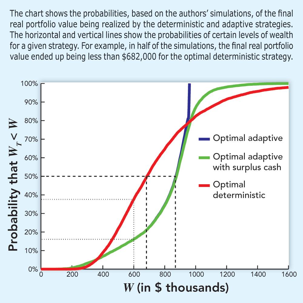
Overall, Figure 2 shows that the optimal adaptive strategy outperforms its deterministic counterpart across a wide range, from probabilities of around 5% to about 80%. In other words, the optimal adaptive strategy is better in all cases except the worst 5% or the top 20%. The underperformance on the high side is due to the de-risking. Effectively, the investor is assumed to be content with achieving the target and has traded off some of the upside in exchange for a measure of downside protection. The degree of underperformance on the high side is mitigated by including surplus cash. This is indicated in the figure, but it is arguably understated since the surplus cash is assumed to be just invested in Treasury bills. If instead it was invested in equities, the curve would be shifted further to the right in this upper range. As for the downside underperformance, it is inevitable. The adaptive strategy always attempts to hit the target, so if realized returns have been very poor, it will invest fully in equities since the target would be otherwise unattainable. If equity returns continue to be poor, the investor following this strategy will suffer further losses. By contrast, the optimal deterministic strategy has some protection against this type of scenario because it will shift at least partly out of equities after the first few years, no matter what has happened.
Summary
Our analysis leads to two main conclusions. First, despite their intuitive appeal, deterministic glide paths do not perform significantly better than the simpler alternative of a constant proportion strategy such as a 60% stock/40% bond allocation. (Note that similar results regarding the relatively poor performance of this type of strategy have been reported in several other studies. See our 2017 study for examples.) Even under the artificial conditions of our synthetic market, the optimal deterministic glide path—which reduces exposure to equities over a set period of time—offers no tangible risk reduction benefits over a simpler constant proportion strategy. This also holds under the more demanding conditions of the historical market.
Second, adaptive strategies appear to be quite promising. We have investigated just one possibility here—shifting to Treasury bills once target wealth is reached—but it offers the same average final value at considerably lower risk in both the synthetic and historical markets. By sacrificing some upside potential in exchange for a degree of downside protection, it achieves outperformance across a wide range of possible outcomes.
The superiority of the adaptive approach is perhaps easily understood through a sports analogy. Consider a football team that commits to playing very aggressively in the first half of the game (e.g., throwing many long passes, never punting on fourth down once across midfield, etc.) so as to build up a lead, and then switching to a very conservative style in the second half to protect the lead (using many running plays to keep the clock moving, always kicking on fourth down, etc.). This could very well be a sensible strategy, provided that the team is successful in building a lead. But what if it isn’t? The deterministic approach characteristic of target date funds implies that the score of the game has no impact on the team’s strategy: Even if the team falls behind in the first half, it will still play conservatively in the second half. A team following an adaptive approach, in contrast, would consider not just the game clock, but also the score. If this team is behind in the second half, it will attempt to catch up by playing aggressively. Of course, this could lead to a loss by an even larger margin. Sometimes “Hail Mary” passes are intercepted and returned for touchdowns. This type of aggressive, but unsuccessful, attempt to recover is why the optimal adaptive strategy is outperformed in the worst 5% of cases by the deterministic strategy.
Obviously, there are return scenarios that will lead to higher final real portfolio values after the fact for one or the other of these strategies. However, without a crystal ball to inform us today of future market returns, the best we can hope for is to tilt the odds of success in our favor. By this standard, the Target Wealth formulation appears to offer a better bet than current alternatives.
Editor’s note: The authors’ aforementioned study, “Target Wealth: The Evolution of Target Date Funds” is available at SSRN (www.ssrn.com) and also from PWL Capital White Papers at www.pwlcapital.com/en/The-Firm/White-Papers.

Related

Portfolio Strategies
Mathematical Support for Rising Equity Glide Paths
Related
Portfolio Strategies
The Advantages of Diversification and Rebalancing
Discussion
FREE REPORT

Get your free copy of our special
report analyzing the tech stocks
most likely to outperform the
market.
Dan Tenney from CT posted over 8 years ago:
Richard Pincombe from CA posted over 8 years ago:
You need to log in as a registered AAII user before commenting.
Log InCreate an account