While successful investors and finance professors alike [as well as AAII] strongly recommend that we not attempt to time the market, it can be frustrating to buy shares only to see a subsequent, rapid price decline, such as that we experienced in the first quarter of 2022. The S&P 500 index, for instance, fell 12.44% through March 14 before recovering to end the quarter down 4.95%.

Can we avoid such corrections by anticipating market volatility? If we had a gauge into the sentiments of market participants, could we predict their decisions to sell shares and adjust our portfolios in advance? Market commentators often point to the S&P 500 Volatility Index, or VIX, as offering such insights, referring to it as “the fear gauge.” But does it hold value?

A Primer on Equity Options

To understand what the VIX is and how its level is determined, a quick primer on equity options is helpful. Suppose you wish to buy a house, financed in part using a mortgage. Your first step would be to get preapproved by the bank, to learn how much you could borrow. You face the risk, though, that interest rates will rise while you are seeking out your ideal property and preparing to close. To help protect you against this risk, the bank will typically offer you the option—for a fee or premium and for a defined time period—to lock in your borrowing rate. At closing, if rates remain unchanged or have dropped, you can borrow at the prevailing rate; if rates have risen, you would exercise your option to borrow at the locked-in rate.

Similar options are available in the equity markets. An investor who is bullish on a stock can pay a premium to purchase a call option that provides the right, but not the obligation, to purchase a share at a specified price (the exercise, or strike price) until a specified expiration date. A bearish investor, on the other hand, can purchase a put option that is similarly defined, but provides for the sale rather than the purchase of the share. (In practice, an option contract relates to the purchase or sale of 100 shares.) At expiration, the value of a call is its payoff, which is the amount, if any, by which the market price exceeds the strike price. Similarly, the value of a put is the amount, if any, by which the market price is below the strike price.

A call option on a stock is said to have intrinsic value if the stock’s current price exceeds the strike price, while a put will have intrinsic value if the stock price is below the strike. Call and put options with intrinsic value are said to be “in the money.” Both options are “at the money” if the stock price equals the strike price, or otherwise are “out of the money” if they have no intrinsic value. Prior to expiration, an option price or premium will be worth its intrinsic value, if any, plus time value that reflects the fact that intrinsic value may increase as expiration approaches.

Factors Influencing Option Pricing

While traders use sophisticated models such as the Black-Scholes to price options, in general an option’s value is the present value of its expected intrinsic value, or payoff, at expiration. The illustration in Figure 1 helps us to make some deductions about the factors that influence the price of a call.

• Stock Price: The greater its current price, S0, the more likely a call option on the stock is to have intrinsic value at expiration. For instance, if its strike is $100, a call on a stock with a current price of $90 is likely to have more intrinsic value at expiration than if the stock price is $50.
• Strike Price: Similarly, the lower the strike price X, the more likely it is that the stock price ST will exceed it, and so the option will have intrinsic value and be in the money at expiration.
• Time: In general, the more time until expiration, the more likely it is that the stock price will appreciate, and so the greater the option value.
• Volatility: The more volatile the stock, the greater the uncertainty about its future price and so the greater the intrinsic value is expected to be at expiration. Note that while it is true that a more volatile stock can also be more likely to decrease significantly in price than a less volatile one, as volatility, or vol, increases, so too does the value of a call.
• Interest Rate: While a stock’s price will typically fluctuate, exhibiting volatility, its price movement over time trends up with interest rates. As rates increase, therefore, so too does the trend in price, increasing the intrinsic value expected at expiration and making a call more valuable.
• Dividends: A stock’s price tends to decrease by the amount of any dividend paid, thereby decreasing the value of a call.

Call and Put Option Parity

While it might not be intuitively obvious, the prices of call and put options are related. Consider two investors, Jack and Jill. Jack’s portfolio consists of one share of Apple Inc. (AAPL) and one Apple put with a $100 strike. If Apple’s price when the option expires exceeds $100—let’s say it is $150—Jack will sell his share for $150. If the stock price falls below $100, however, he can use the put option to sell it for $100.

Meanwhile, Jill owns a $100 strike price call option on Apple stock, with the same expiration date as Jack’s put. She also owns a $100 Treasury bill, which she will redeem at expiration for $100. If the stock has risen to $150, she can use the call option to purchase a share for $100, and then sell the share for $150. If the stock falls below $100, however, the call option will be worthless. She will still receive $100 from redeeming the T-bill. Jill’s portfolio is worth the same as Jack’s, in both up and down markets, and so must have the same value today. We can use that relationship to deduce the value of a call option from that of a put, and vice versa.

Incidentally, we can also infer from this relationship the surprising result that a stock’s expected growth rate does not affect the value of the option. If it did, call options on high-growth stocks should become more valuable as the projected growth rate increases and put options should become less valuable. But that would break the parity relationship, and so we can conclude that a stock’s assumed growth rate is not relevant to option pricing. Instead, for option pricing purposes, stocks are assumed to grow at the risk-free, or T-bill, rate.

Stock Price Volatility

Suppose I offered you an investment that promised an average payout of $10 every year for, say, 10 years. I could honor that promise by paying you exactly $10 every year. Let’s refer to this as Case A. Alternatively, I could pay you $9 some years and $11 other years (Case B). Or I might pay you $0 some years and $20 in other years (Case C). In each case, however, the average or mean annual payment would be $10. Most people, I expect, would prefer Case A—the continual stream of $10—to Case B. Case C would likely be the least preferred. That is because investors, in general, prefer stable or predictable cash flow streams to those that vary. In Case C, the payments fluctuate the most and have the greatest volatility.

In general, volatility reflects how far on average each observation is from the mean. In Case A, each payment is exactly $10, so the average distance from the mean of $10 is $0. In Case B, each payment is $1 from the mean of $10, so the average distance is $1. Finally, in Case C, each payment is either $0 or $20, so the average distance from the mean is $10. In practice, rather than measuring dispersion using average absolute distance from the mean, the volatility of a stock price is typically expressed using standard deviation, which is the square root of the average of the squared distances from the mean.

Implied Volatility in Options Prices

An interesting feature of option pricing is that it depends on how volatile stocks will be in the future. But that, of course, is unknown to us since we don’t have a crystal ball. All that we know for certain is how the stock’s historical prices have varied, as measured by their standard deviations, which we refer to as their historical volatility. This is what traders typically use as an initial input in their option pricing models.

An investor looking to hedge the risk that a stock price will decrease might purchase a put option with the factors listed above, including historical volatility, being used by a trader to determine the option’s “correct” price. However, as more and more investors purchase the same option, increased demand will start to drive its price up. Note that this can happen without the underlying stock price moving or time passing—in short, none of the option pricing factors moving. How then can the model generate an option value that matches the new, increased, market price? By increasing the volatility assumption fed into the model: The level of volatility that must be fed in so that the model outputs an observed market price is known as the implied volatility.

Market Sentiment, Options and Implied Volatility

Because of option parity, generally, the implied volatility for put and call options is very close. But consider investors concerned about a broad market correction.

They are likely to purchase put options on the S&P 500, driving up option prices and, therefore, implied volatility. Their motivation to hedge is based on a fear that prices will decrease sharply—in other words, that prices will become more volatile in the near term, which is exactly what an increase in implied volatility suggests.

The VIX and the Implied Volatility of the S&P 500

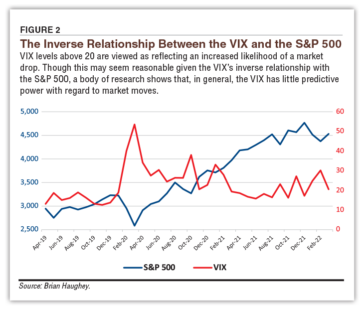
CBOE Global Markets publishes the VIX, which is a volatility index based on the implied volatility of 30-day options on the S&P 500. Market observers use the VIX to gauge market sentiment by reading the levels of implied volatility in the broad market. Indeed, the VIX is often referred to as the “fear gauge.” VIX levels above 20 are viewed as reflecting an increased likelihood of a market drop. At first glance, this use of the VIX seems reasonable, with Figure 2 showing that there is an inverse relationship between the VIX and the S&P 500.

For investors who wish to time the market, however, this use of the VIX is not that useful. A body of research shows that, in general, the VIX has little predictive power regarding market moves. In other words, the market is already starting to move at the same time that the level of implied volatility increases. The VIX can be useful, however, as an alternative means to hedge against equity risk. While the index itself is not traded, investors concerned about a potential drop in the S&P 500 can purchase options or futures contracts on the VIX.

The VIX: Pay Attention to Its Moving Average

Market watchers who use the VIX as a predictive tool tend to focus (mistakenly, in my view) on its absolute level, and whether, for instance, it is above or below 20. If we make some simplifying statistical assumptions given that there are about 250 trading days in a year and that the square root of 250 is close to 16, we are led to the Rule of 16. When the VIX level is 20, for instance, the Rule of 16 indicates that the daily change in the price of the S&P 500 won’t exceed 1.25% (20% ÷ 16 = 1.25%) about two-thirds of the time. One-third of the time, however, the daily price move will be greater. At the VIX’s record high of 82.69 on March 16, 2020 (note that Figure 2 shows end-of-month levels of the VIX), the options market was pricing in about a one-third chance that the S&P 500 would move more than 5% (82.69% ÷ 16) on a given day.

The power of the VIX, in my opinion, lies more in its relative, or comparative, level. For instance, an increase in the VIX above its moving average could be considered a bearish signal. A decrease below the moving average could be considered a bullish signal. While some traders watch moving average crossovers of the S&P 500 to make buy and sell decisions, on occasion crossovers in the VIX can provide earlier signals, particularly after sell-offs.

In Figure 3, for instance, we can see that the actual VIX level (in red) dropped below the five-day simple moving average (black dotted line) on January 27, 2022, just as the S&P 500 (blue) begins to turn up. Similarly, the VIX signaled the beginning of a recovery on March 9, 2022. In both cases, the VIX signal came slightly ahead of signals produced by the five-day moving average on the S&P 500.

Use the VIX for Insight, Not Market Timing

While options are powerful tools for both hedging and speculation and can provide insight into market sentiment particularly through the VIX, they don’t offer much value to market timers. Indeed, Peter Lynch, perhaps the most successful fund manager of all time, strongly advocated against seeking to time the market, “People spend an unbelievable amount of mental energy trying to pick what the market’s going to do, what time of the year to buy it. It’s just not worth it.” I would echo his advice, and point out that for most investors, a regular pattern of investing in the market is the recommended strategy.

Although watching the VIX can provide a perspective on fear in the market, I would suggest that it is not enough to influence your investing strategy, at least as it is commonly used. However, investors who follow a disciplined strategy of making regular, periodic investments may benefit by using a VIX crossover strategy during a market sell-off to determine whether waiting a few days might be advantageous.

Related

Investor Professor

Online Exclusive: What Is the Put-Call Ratio?

Related

Dispatches

What Triggers Market Jumps?

Related

Trading Strategies

Missing the Market's Worst and Best Months