

Related

Portfolio Strategies
A diversified portfolio not only increases return relative to risk, it can also boost the amount of income provided by RMDs.

Think of “asset allocation” as a portfolio recipe.
Recipes naturally involve the blending of different amounts of various ingredients—usually followed by some type of cooking or baking. If we follow the recipe, the outcome is generally quite predictable. Where we purchase the ingredients is less important than knowing how much of each ingredient to use. Said differently, the recipe is more important than the source of the ingredients.
Investment portfolios operate the same way. We blend various asset classes together according to certain allocations. We then “cook” the portfolio for a period of years. We might need to stir it occasionally, which is analogous to rebalancing the portfolio. In the end, the asset allocation largely determines the outcome as opposed to where we purchased the ingredients. Whether we purchased mutual funds or exchange-traded funds (ETFs) from Vanguard or Schwab is not as important as the asset allocation model—or portfolio recipe.
In this article, I examine a number of asset allocation recipes and how they performed over the past 47 years (from January 1, 1970, to December 31, 2016).
The first recipe is 100% cash (Table 1). Cash is only one asset class and therefore does not represent an asset allocation model (which implies at least two asset classes) by itself. However, as many investors often hide out in cash when they are afraid of the stock markets or worried about bonds, it’s worth examining the performance of cash over the past 47 years. As can be seen, the average annualized nominal return of a 100% cash investment was 4.97% with a standard deviation of annual returns of 3.54%. (Standard deviation shows how much returns have typically varied from their average.) The worst-case three-year cumulative nominal return (often referred to as “drawdown”) was a positive 0.13%.
The average 10-year rolling nominal return for cash was 5.48%. This may come as a surprise, given such low interest rates for the past nine years. It’s important to recognize that a nominal return does not factor in the impact of inflation [as measured by the consumer price index (CPI)].
Real returns adjust performance to reflect the impact of inflation. On a real-return basis, the performance of cash looks quite a bit more modest: a 47-year return of 0.90%, a negative 6.51% worst case three-year cumulative real return, and an average 10-year rolling return of 1.32%. Real returns represent reality because they account for the loss of value caused by inflation. Put another way, the amount of goods and services cash can buy when its value is adjusted for inflation barely increases over the long term; it has even decreased during certain periods.
We now move up the asset allocation food chain to a 50% bond/50% cash portfolio. This portfolio represents actual asset allocation, albeit a very conservative approach. The nominal 47-year return was 6.33%, while the real return was 2.21%. The difference in worst-case three-year cumulative return is quite dramatic: 2.29% in nominal terms and –14.29% in real terms. This reveals that fixed-income portfolios may look like a safe haven when we ignore inflation, but are not so protective once inflation is accounted for.
The next portfolio is a 25% stock/75% bond and cash portfolio. Its specific allocation is 20% cash, 55% bonds, 15% large-cap U.S. stock and 10% small-cap U.S. stock. Not surprisingly, performance increases, volatility increases and the worst-case three-year return represents a bigger drop.
The fourth portfolio is a broadly diversified, multi-asset portfolio. This portfolio used seven different asset classes in equal portions (14.29% each) and was rebalanced annually. The asset classes included large-cap U.S. stock, small-cap U.S. stock, non-U.S. developed stock, real estate, commodities, U.S. bonds and cash. The actual historical returns from the following indexes were used in the analysis: S&P 500, Russell 2000, MSCI EAFE (Europe, Australasia and the Far East), Dow Jones U.S. Select REIT, S&P GSCI (Goldman Sachs Commodity Index), Barclays Capital U.S. Aggregate Bond and 90-day U.S. Treasury bill.
Table 1. Comparison of Returns for Five Allocations (1970–2016)
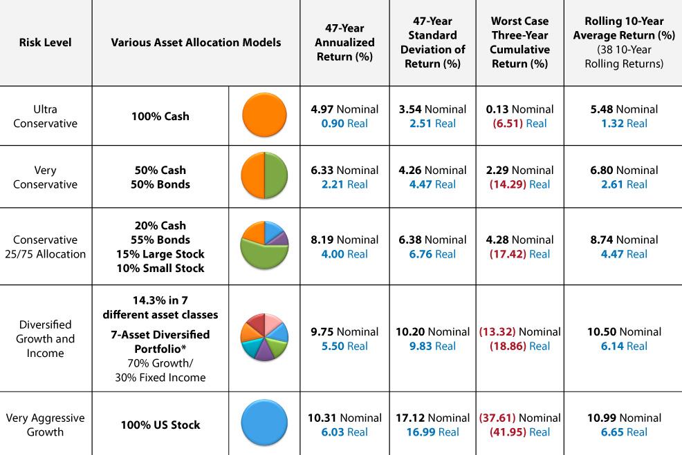
The multi-asset portfolio generated a 47-year average annualized nominal return of 9.75% with a standard deviation of 10.20%. Relative to the 25/75 portfolio, returns for the seven-asset portfolio were higher, though so was the volatility of returns. The worst-case three-year decline of –13.32% was considerably worse than the +4.28% gain the 25/75 portfolio realized as its worst-case three-year cumulative return. However, when evaluated in “real” inflation-adjusted terms, the 25/75 portfolio had a worst-case three-year decline of 17.42%, which is nearly the same as the multi-asset portfolio. This suggests that a portfolio with more ingredients (in particular real estate and commodities) has historically offered better inflation protection than a portfolio lacking those asset classes.
Finally, we examine a 100% stock model. As with the 100% cash model, this does not represent an asset allocation model because it only includes one asset class. But, inasmuch as large-cap U.S. stock is a very prominent asset class and serves as a performance benchmark, it is reviewed here. The 47-year average annualized nominal return of U.S. large-cap stocks was 10.31%, and 6.03% in real terms. The standard deviation of an all-U.S. stock portfolio was basically 17% in either nominal or real terms. The worst-case three-year decline was a troubling –37.61% in nominal terms and –41.95% in real terms. That’s tough to stomach. Finally, the average rolling 10-year nominal return was 10.99% versus 6.65% in real terms.
What are the advantages of building a diversified multi-asset portfolio? Compared to a 25/75 portfolio, a seven-asset equally-weighted portfolio produced 150 basis points higher real return over this 47-year period. The volatility (using real annual returns) increased by just over 45%, but the worst-case three-year drawdown was nearly the same. The average rolling 10-year real return for the seven-asset portfolio was 167 basis points higher than the 25/75 portfolio.
Compared to a 100% large-cap U.S. stock investment, a multi-asset portfolio had a 47-year average annualized real return that was about 9% lower, but as compensation was 42% less volatile. The worst-case three-year decline was less than half as bad as it was for the all-stock portfolio. Finally, the average rolling 10-year real returns were within 51 basis points of each other, which is important because very few investors wait around for 47 years to evaluate how they’re doing.
For retirees or those nearing retirement, the real test of a portfolio and the asset allocation model that drives it takes place when money is being systematically withdrawn. This is sometimes called the “distribution phase” of a portfolio. Very simply, it is a portfolio torture test. The sequence of returns—meaning the order in which returns occur—becomes critical during this period, since negative returns in the early years of withdrawals can shorten how long the portfolio lasts. However, the required minimum distribution (or RMD) is a natural defense against portfolio failure. The RMD may be viewed by many retirees as the bad guy. The analysis presented next may change that perception.
RMDs must be taken from most retirement accounts [traditional IRAs, 401(k) plans, Roth 401(k) plans, SEPs, 403(b) plans, etc.; Roth IRAs are exempt from the rule, however.] The amount of the annual mandatory distribution is determined by the RMD numbers from the Uniform Lifetime Table (for retirees whose spouse is not more than 10 years younger than themselves). The amazing part is that the mathematics of the RMD virtually guarantee that a portfolio cannot be liquidated within 45 years. The absolute dollar amount of the RMD may not be large enough to meet a retiree’s spending needs, but if speaking only in terms of retirement portfolio survival, the RMD works for more than 45 years.
The first RMD divisor from the Uniform Lifetime Table is 27.4 (www.irs.gov/pub/irs-tege/uniform_rmd_wksht.pdf). Each divisor is used to calculate each year’s distribution from the portfolio. If the account balance was $1 million at the end of the prior year and the retiree is at least 70½ years old, the required minimum distribution would be calculated as $1,000,000 ÷ 27.4 = $36,496. The divisor of 27.4 is the equivalent of a 3.65% withdrawal rate. In year two the RMD divisor is 26.5. The year-end account balance from year 1 would be divided by 26.5 to determine the required minimum distribution. The divisor of 26.5 is the equivalent of a 3.77% withdrawal rate.
The RMD–based annual withdrawals start out as relatively small percentages and then escalate to 10% when the retiree hits the age of 92. By the age of 100, the annual withdrawal rate based on the RMD is almost 16%. At 110, the RMD requires that a retiree withdraw over 32% of the prior year’s ending account balance. Despite the dramatic withdrawal percentages later in life, the RMD methodology preserves a portfolio until age 116. Granted, the size of the withdrawals in the latter years will be ridiculously small, but the math of the RMD is designed to preserve the portfolio for 47+ years.
Let’s now examine several different retirement portfolios and how they fared using RMD-based annual withdrawals. Over the 47-year period from 1970–2016 (corresponding to a retiree from age of 70 to 116). The four portfolios being analyzed are the 100% cash portfolio, the 50% cash/50% bond portfolio, the 25% stock/75% bond and cash portfolio, and the seven-asset diversified portfolio. The starting balance was assumed to be $1 million at age 70 when the RMD begins.
As shown in Figure 1, all four portfolios had the same initial withdrawal in the first year of $36,496 (which is the prior-year balance of $1,000,000 divided by the RMD divisor of 27.4, which works out to be a withdrawal rate of 3.65%). After the first year, all subsequent annual withdrawals are a function of how well each portfolio performed in the prior year. As can be seen, all four retirement models had positive annual withdrawals all the way through age 116 IF withdrawing ONLY the amount of money mandated by the RMD—that is, the required minimum distribution. In each case, the annual withdrawal converges to nearly zero at the age of 116.
Figure 1. Annual Withdrawal Amounts Based on the RMD
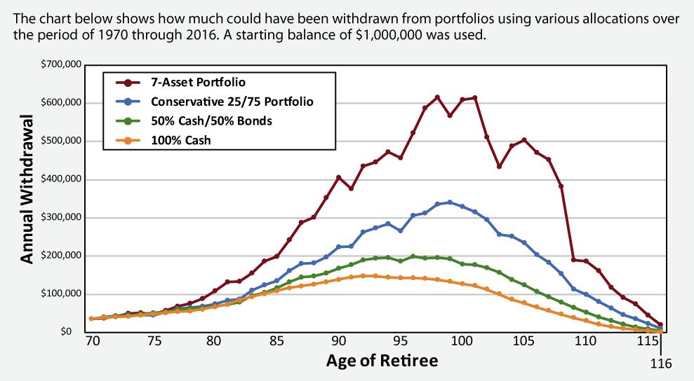
The seven-asset portfolio is clearly the better performer based on its more diversified and growth-oriented ingredients. In fact, between the ages of 96 and 102 each annual withdrawal was in excess of $500,000 based on the RMD divisor at those ages. If the retiree lived to be 116 years old, nearly $13 million would have been cumulatively withdrawn from the seven-asset portfolio. If the retiree was always invested in the 100% cash portfolio, a total of $3.8 million would have been withdrawn over the 47-year period.
In fact, even a portfolio with 0% annual return (not shown in the graph) generated positive withdrawals each year, though much smaller. A total of $999,853 would have been withdrawn over the 47-year period, leaving a balance of $163 when the retiree was 116 years old.
The year-to-year ending account balances of each portfolio converge to zero when the retiree is 116 years old. Again, this analysis assumes the retiree never withdrew more than the RMD each year. Note that the seven-asset portfolio had year-ending account balances over $4 million when the retiree was between the ages of 88 and 97. After that age, the RMD divisor becomes increasingly more demanding and the portfolio begins a downward path toward liquidation regardless of the portfolio design.
While interesting, the analysis presented thus far is based on a specific time period from 1970 to 2016. This is only one sequence of returns that a retiree could have experienced. Moreover, it is a 47-year time frame, which is much longer than any retiree will likely experience. To account for the variation in portfolio performance caused by different sequence of returns (one of the primary risks that retirement portfolios are exposed to) and a more typical retirement period of 25 years, I analyzed the performance of each portfolio over rolling 25-year periods. Between 1970 and 2016 there were 23 rolling 25-year periods: 1970–1994, 1971–1995, and so on.
The results of the rolling period analysis for five portfolios, including a 100% large-cap stock portfolio, are summarized in Table 2. Each portfolio survived for at least 25 years in every rolling period, but we already knew that would be the case based on the mathematics of the RMD methodology. More relevant is the average ending balance at the end of each 25-year period, the average amount of money that the retiree was able to withdraw each year and the average amount withdrawn in total over each 25-year period. The 100% large-cap U.S. stock portfolio was included in this rolling period analysis for illustrative purposes, though it would not be suggested in actual practice inasmuch as it does not represent a broadly diversified portfolio. Moreover, under different assumptions (such as when not basing withdrawals solely on the minimum annual RMD), it often does not perform as well as a more diversified portfolio (such as the seven-asset portfolio).
Table 2. Retirement Portfolios With RMD-Based Annual Withdrawals

Raw data source: Steele Mutual Fund Software, calculations by author. Analysis completed by using the Retirement Portfolio Survival Analyzer Excel spreadsheet, developed by the author. Past performance does not guarantee future performance. The multi-asset portfolios were rebalanced at the start of each year.
*The 7-asset portfolio equally weights the S&P 500, Russell 2000, MSCI EAFE, Dow Jones US Select REIT, S&P GSCI, Barclays Capital US Aggregate Bond and 90-day U.S. Treasury bill.
The RMD methodology is a safety net that retirees should not ignore. Building a retirement portfolio that is too conservative ignores the mathematics designed to preserve the portfolio. In other words, if the retiree only withdraws the minimum each year, they can stop worrying about driving their account balance to zero within their lifetime. There will still be money in the portfolio if a retiree only withdraws the minimum each year.
Retirees do, however, need to consider whether or not a RMD-based withdrawal will be large enough to meet their spending needs each year. That, of course, is a function of two variables: (1) having a large enough retirement account balance AND (2) building a diversified portfolio that generates the needed return to prudently grow the portfolio.
The first issue can’t be fixed once a retiree hits retirement, but retirees can certainly build an appropriate growth and income retirement portfolio that is built for the long run—because that is exactly what retirement is for a growing number of people.
Portfolio Strategies

Portfolio Strategies

Financial Planning

George Bussey from HI posted over 9 years ago:
Richard Huff from MD posted over 9 years ago:
HOWARD from CA posted over 9 years ago:
Jim from MI posted over 9 years ago:
Jean from IN posted over 9 years ago:
Swain Sheppard from SC posted over 9 years ago:
Richard Vroman from CA posted over 9 years ago:
David Lewis from UT posted over 9 years ago:
Tony Hausner from MD posted over 9 years ago:
William Wright from WI posted over 9 years ago:
Richard Vroman from CA posted over 9 years ago:
William Wright from WI posted over 9 years ago:
John from CO posted over 9 years ago:
Craig Israelsen from UT posted over 9 years ago:
Craig Israelsen from UT posted over 9 years ago:
Craig Israelsen from UT posted over 9 years ago:
DEM from Arizona posted over 6 years ago:
You need to log in as a registered AAII user before commenting.
Log InCreate an account