

Related

Small Cap Value Investing
Small-cap stocks thrive during periods of expansive monetary policy, while returns for large- and small-cap stocks are lower during restrictive periods.

We all know that investors and the financial media alike have become fixated on the actions of what was one time a very obscure body, the Federal Reserve Board of Governors.
And it isn’t merely the financial media that increasingly focuses on the actions (or inactions) of this august body. Former Fed chairman Alan Greenspan became a celebrity, former Fed chairman Ben Bernanke is in high demand as a public speaker, and current Fed chair Janet Yellen was named Time Magazine’s “Person of the Moment.” It is obvious that Main Street also pays attention to the actions of the Federal Reserve.
Financial markets seemingly move on mere speculation that the Fed might increase, decrease or even leave key interest rates unchanged in the near future. Headlines such as “Fed Up: Do Rising Rates Matter to Stocks?,” “The Fed Poisons the Stock Market,” “What Happens to Stocks When Interest Rates Rise?” and “Investors Price in Another Fed Rate Increase After Jobs Data” have become all too commonplace in media outlets.
There is also widespread disagreement on what rising or falling policy rates means for the markets. Some market pundits rationalize that rate hikes by the Federal Reserve are good news for investors because they signal that the economy is gaining strength and corporate earnings will likely increase with a more robust economy. People in this camp believe that stocks outperform in a rising interest rate environment. Others contend that rising rates are bad news for the stock market: As companies’ borrowing costs increase, bond yields rise and bonds become more attractive to investors vis-à-vis stocks. These investors interpret rate hikes as foreboding lower returns to equities.
So, which camp is correct? As three researchers who have studied Fed policy and capital market returns for nearly 25 years, we prefer to look at the hard, empirical evidence. As Detective Sergeant Joe Friday from the television series Dragnet is famously misquoted as saying, “Just the facts, ma’am.” We also focus on long-term returns and not short-term reactions to announcements of changes in Fed monetary policy. While short-term reactions receive a great deal of attention, it is the long-term market performance that is of greatest interest to the true investor.
In this article, we summarize how stocks—particularly small-cap stocks—have performed during different Federal Reserve rate environments. Now, that doesn’t mean that the market will perform exactly as it has in the past with respect to Fed policy. But, as the saying often attributed to Mark Twain goes, “History doesn’t repeat itself, but it does rhyme.” We think this information is valuable for investors to consider when formulating an investment strategy or considering potential tactical asset allocation adjustments in response to changes in Fed monetary policy.
In our published research papers and in our recently published book “Invest with the Fed: Maximizing Portfolio Performance by Following Federal Reserve Policy” (McGraw-Hill, 2015), we developed a measure of monetary conditions that considers two key Fed policy rates: the discount window primary credit rate (more popularly known as the Fed discount rate), and the federal funds rate. We believe there is substantial information in each rate and utilize both to characterize the Federal Reserve monetary environment. The benefit of our classification scheme is that it relies solely on these two rates, is not subject to interpretation and can be easily monitored by investors. There is also no ambiguity. All one needs to properly classify the monetary environment is to monitor these two rates on a monthly basis.
It is important to note that our classification scheme is not predicated on the level of interest rates—whether policy rates are historically high or low. We have found in previous studies that it isn’t so much the level of rates as it is the direction of changes in rates that is strongly associated with security returns. In other words, it isn’t whether rates are high or low in comparison to historical levels, but whether policy rates are rising or falling.
The discount rate is the rate the Fed charges on loans to member banks. It is set by the Federal Reserve and often remains unchanged for months or even years at a time. In fact, at the time of this writing it was a miniscule 0.75% and had been at that same level since February of 2010. The discount rate is viewed by many observers as a symbolic rate—an indication of the Fed’s long-term (or broad) policy objectives. Specifically, changes in the discount rate are viewed as signaling the Fed’s long-term intentions—we reference these changes as indicators of the Fed’s monetary policy stance.
The federal funds rate is the rate on loans that banks extend to each other. Federal funds loans are generally very short-term in nature and are considered as part of the market for overnight money. While the Fed doesn’t set the federal funds rate, it does set a target level for that rate. We interpret the federal funds rate as reflecting the short-term stringency of Fed policy. It indicates the degree of constraint the Fed is applying in the short-term market for funds.
We look at the last monthly change in the direction of the rate to classify the environment. If the last monthly change was a decrease, we classify the environment as expansive. Conversely, if the last monthly change was an increase, we classify the environment as restrictive. At the time of this writing, the last monthly change in the discount rate occurred in February 2010 when the rate increased from 0.50% to 0.75%. Thus, with respect to broad monetary stance, we would say that the Fed is in a restrictive environment. And the policy classification will remain restrictive until the Fed discount rate is lowered.
Given the extremely low interest rates and expanding money supply over the last several years, you may question whether the Fed’s broad policy has really been restrictive since February 2010; we agree with that sentiment. However, what the measure indicates is that the Fed has signaled its intention to move toward a restrictive policy when conditions permit. We rely on the second policy variable (as described below) to identify when the Fed actually begins implementing its signaled policy.
Our second Fed policy variable identifies the degree of monetary stringency actually being applied by the Fed. The average federal funds rate was 0.12% for December of 2014 and decreased to 0.11% in January of 2015. Thus, at the time of the writing of this article, we would consider the stringency of monetary policy to be expansive, as the last change in the federal funds rate was a decrease.
Now, the key to our classification scheme is to look at both interest rates to classify the overall monetary environment. If both are restrictive, then we classify the overall monetary environment as restrictive. Likewise, if both are expansive, we classify the overall monetary environment as expansive. If one of the rates is expansive and the other is restrictive, we classify the overall monetary environment as indeterminate. Table 1 provides a summary.
Table 1. Classification of Monetary Policy Environment

According to our classification scheme, at the time of the writing of this article, the monetary environment would be considered indeterminate as the stance of the Fed is restrictive, while the stringency of the Fed is expansive. To monitor these rates, readers can refer to the Federal Reserve’s website, particularly its database of historical interest rates: www.federalreserve.gov/releases/h15/data.htm.
Since 1966 the Fed has followed an expansive monetary policy about one-third of the time, a restrictive monetary policy one-third of the time, and an indeterminate monetary policy about one-third of the time. Thus, when we look at how the markets have fared during different monetary environments, readers can rest assured that the results are not driven by small sample sizes.
What does the evidence suggest regarding stock market performance during different monetary policy environments? Are rising Fed policy rates best for stock market performance, or are falling rates a boon to stocks?
Table 2 shows the results for large-cap stocks (as proxied by the S&P 500 index) during different Fed monetary policy periods. The evidence clearly shows that when the Fed is in a rate-lowering mode, on average, the markets have prospered, and when the Fed is raising policy rates the markets have struggled. The table also includes the inflation rate during these monetary policy periods. Once you consider inflation, the differences in the real returns to large-cap stocks during different monetary policy periods is even more dramatic. The stark difference in returns is highlighted by the finding that the real return on the S&P 500 during expansive monetary conditions is 12.32% (15.18% – 2.86%), while during restrictive conditions it is only 0.66% (5.74% – 5.08%).
Table 2. Large-Cap Stock Performance During Different Monetary Conditions
Large-cap stock performance under different monetary conditions between January 1966 and December 2014. All returns and the inflation rate are annualized.*
|
|
Expansive Monetary Conditions |
Indeterminate Monetary Conditions |
Restrictive Monetary Conditions |
|
|
|||
|
|
|||
| Large-Cap Stock Return (%) | 15.18 | 11.46 | 5.74 |
| Inflation Rate (%) | 2.86 | 4.17 | 5.08 |
*We follow the standard approach of annualizing mean monthly returns by multiplying the monthly value by 12.
Some recent research suggests that the widely documented small-firm effect (the theory that firms with a small market capitalization outperform large-capitalization companies on a risk-adjusted basis) either no longer exists or is less prevalent. Some market observers—notably, Jeremy Siegel—contend that once the small-firm effect became well documented, investors priced the relationship away. Our objective is not to prove or disprove the small-firm effect; instead, we provide evidence that the small-firm effect is influenced by Fed monetary policy.
Table 3 shows returns across the market-capitalization spectrum during different Fed monetary policy periods. The average annual returns are derived from the size-based portfolios that are reported on the Kenneth French website; we use value-weighted returns. The portfolios are based on New York Stock Exchange (NYSE) breakpoints. For example, the “small quintile” includes stocks with a market cap that is below the 20% ranking of NYSE stocks. See the French website (http://mba.tuck.dartmouth.edu/pages/faculty/ken.french/) for a more complete description of the size-based portfolios.
Table 3. Annual Return by Market Capitalization: January 1966 to December 2014
Performance for various company sizes under different monetary conditions between January 1966 and December 2014. All returns and the inflation rate are annualized.*
|
|
All Monetary Conditions |
Expansive Monetary Conditions |
Indeterminate Monetary Conditions |
Restrictive Monetary Conditions |
|
|
||||
|
|
||||
| Small-Company Quintile Return (%) | 13.45 | 28.39 | 9.25 | 5.14 |
| Quintile 2 Return (%) | 13.61 | 24.80 | 11.97 | 5.75 |
| Quintile 3 Return (%) | 13.30 | 22.96 | 12.30 | 6.08 |
| Quintile 4 Return (%) | 12.71 | 20.23 | 12.33 | 6.65 |
| Big-Company Quintile Return (%) | 10.32 | 14.36 | 11.42 | 5.66 |
| Inflation Rate (%) | 4.09 | 2.86 | 4.17 | 5.08 |
*We follow the standard approach of annualizing mean monthly returns by multiplying the monthly value by 12.
As you can see from Table 3, there is a pronounced small-firm effect during expansive monetary policy conditions. The real return from the small-quintile portfolio is a staggering 25.53% (28.39% minus the inflation rate of 2.86%). This compares with a real return from the S&P 500 during expansive monetary conditions of 12.32%, as indicated in Table 2. The small-quintile portfolio actually underperforms the S&P 500 during indeterminate monetary policy conditions by 2.21%. Furthermore, the returns for the small-cap portfolio barely keep pace with inflation during restrictive monetary policy periods, offering a real return of only six basis points.
From Table 3, the small-firm premium, which is commonly calculated as the difference in returns between the small and big portfolio, differs dramatically across the three monetary periods. The small-firm premiums are 14.03% (28.39% – 14.36%), –2.17% (9.25% – 11.42%) and –0.52% (5.14% – 5.66%), respectively, for the expansive, indeterminate and restrictive monetary periods. Thus, a leveraged strategy that was long small stocks and short big stocks would have excelled during expansive conditions, but would have bombed during indeterminate and restrictive conditions.
An examination of the return differences across the monetary environments also yields some surprising results, particularly for the small-cap portfolio. Incredibly, the difference in returns between expansive and restrictive periods for the small-cap portfolio is enormous. On a nominal basis, during expansive conditions relative to restrictive conditions, the small-cap portfolio returns an extra 23.25% (28.39% – 5.14%). On a real return basis, the difference in returns for this portfolio is even more compelling at 25.47%.
In contrast, the difference in returns between expansive and restrictive periods for the large-cap (big) portfolio is relatively moderate. On a nominal basis, the extra return offered during expansive versus restrictive monetary periods for the large-cap portfolio is only 8.70% (14.36% – 5.66%). On a real return basis this difference is 10.92%.
You may be tempted to attribute the extraordinary returns earned by the small-cap portfolio during expansive conditions to an unusual level of risk during expansive conditions. After all, higher risk should be rewarded with higher returns.
Such is not the case, however, as the small-cap portfolio actually exhibits more risk during restrictive conditions (the standard deviation, which is a measure of the variance in returns, is 23.55%) than it does during expansive conditions (a standard deviation of 22.20%). The differences in risk across monetary environments for the other four portfolios are comparable.
Due to the lack of any significant risk differences across monetary environments, we choose to omit risk metrics from the analysis for conciseness purposes.
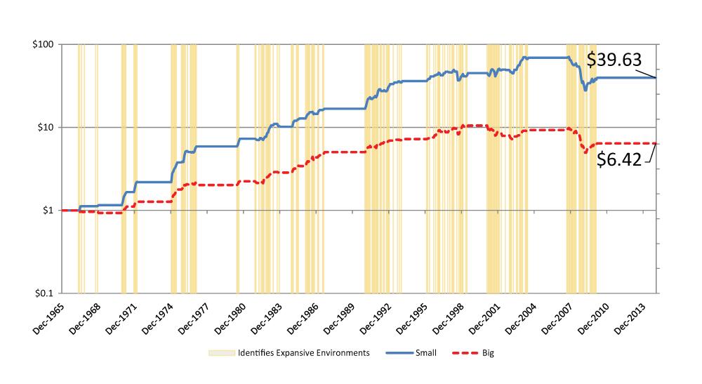
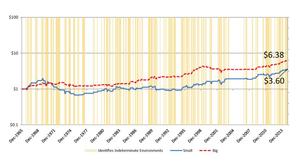
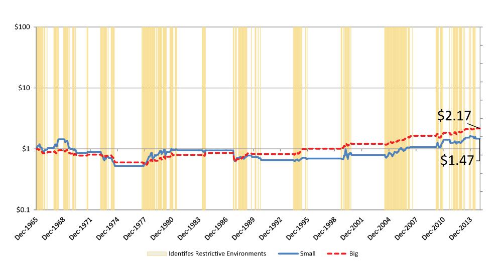
In order to illustrate the monetary-based return pattern over time, we use the quintile portfolios to generate plots of cumulative wealth indexes for each of the three monetary periods. The wealth indexes represent the growth of $1 invested in either the small-cap portfolio (Small) or the large-cap portfolio (Big). In Figure 1, we plot the cumulative wealth index relative to expansive monetary conditions for each of the two portfolios. The plotted values in Figure 1 represent the growth in $1 if the investment was held only during expansive monetary conditions. During indeterminate and restrictive monetary periods, the two portfolios are assumed to earn no return.
As shown in Figure 1, the $1 invested in the small-cap portfolio during expansive monetary conditions grows to $39.63 by the end of the study period, whereas the same dollar invested in the large-cap portfolio during expansive conditions grows to only $6.42. Remember, these plots represent the growth that accrues to the two portfolios during expansive monetary conditions only. During indeterminate and restrictive conditions (the unshaded portion of the figure) the plots remain horizontal (returns are set to zero). By plotting the indexes over the entire sample period, the timing of the growth in value is made apparent. Specifically, it becomes clear that the small-cap portfolio grows considerably throughout the study period, meaning growth occurs during early expansive monetary periods, mid-sample expansive periods and recent expansive periods. The one glaring exception to this growth occurs during the 2008 financial crisis, when it appears that even an expansive monetary policy was unable to stimulate portfolio growth in the small-cap portfolio. This perhaps isn’t a big surprise given the unprecedented nature of the 2008 crisis. In contrast to the small-cap portfolio, the large-cap portfolio grows strongly in one of the early expansive periods, but from then on experiences fairly limited growth in subsequent expansive periods. Overall, the result is an increasing spread between the small-cap wealth index and the large-cap wealth index as we progress through time. This observation supports the existence of a fairly consistent small-firm premium during expansive monetary conditions.
Figure 2 follows the format of Figure 1 in reporting growth for the cumulative wealth indexes during indeterminate monetary periods. In Figure 2, we now assign a zero return for each portfolio during expansive and restrictive monetary periods. Surprisingly, Figure 2 shows that during indeterminate monetary periods, the cumulative growth is greater for the large-cap portfolio than it is for the small-cap portfolio. In particular, “Big” grows from $1 to $6.38 during indeterminate periods, whereas “Small” grows from $1 to only $3.60 when conditions are indeterminate. Based on the spread between the indexes, the difference in performance between the two portfolios appears to be attributed mostly to a short period early in the sample and an interval around the middle-to-latter portion of the sample period. This is apparent as the spread widens considerably from the early 1970s to mid-1970s and again starting in the late 1980s through the 1990s. Otherwise, there appears to be no recognizable pattern in outperformance for either of the two portfolios over the sample period. Clearly, there is no reliable pattern in the difference in performance of the portfolios during indeterminate conditions. This result contrasts sharply with the consistent outperformance of small caps during expansive monetary periods as shown in Figure 1.
Finally, Figure 3 reports the growth in the wealth indexes during restrictive monetary conditions. The graph clearly shows that during restrictive conditions both portfolios perform relatively poorly throughout the entire sample period. The large-cap portfolio value grows to only $2.17, which beats the small-cap accumulated value of only $1.47. From the plots, it is clear that the outperformance of Big is not a consistent phenomenon, but is isolated to the period starting in about 1990 through the early to mid-2000s. Again, this appears to be a minute and unreliable pattern.
The evidence we provide here shows that the small-firm effect is indeed alive and well, but it appears to be entirely concentrated in expansive monetary policy periods. Why would this be the case?
There are obviously strong reasons to believe that the Federal Reserve has the ability to influence the overall performance of the stock market. After all, the Fed controls the money supply and when funds are made more readily available, the stock market generally prospers because of increased economic activity and easier (and cheaper) access to financial capital. But why are the returns to smaller stocks much more dependent upon monetary conditions than the returns to larger-capitalization firms?
We believe there are two alternative economic justifications for this observation. First, while all firms benefit from increased fund availability during expansive monetary policy periods, we believe that smaller firms are generally more sensitive to credit conditions than their larger counterparts. In particular, in tighter monetary policy conditions, smaller firms have greater difficulty acquiring funds via either bank loans or bond issuance than large firms. Conversely, in expansive monetary periods small firms benefit from the availability of capital to a greater degree than larger firms. In general, relative to small firms, large firms have more consistent access to alternative sources of funds regardless of the degree of constraint in monetary conditions/fund availability.
A second explanation relates to borrowing by investors. During expansive monetary conditions, money is more readily available to investors, so speculators are more willing to acquire and hold smaller stocks. Relative to larger firms, the stocks of smaller firms are generally less liquid and are subject to greater margin constraints. Therefore, when funds are expected to be readily available, speculators will allocate a greater proportion of their portfolio to small stocks, which drives small stock prices up. When fund availability is in doubt, speculators are more likely to choose to hold a greater proportion of large-firm stocks.
Overall, based on these two alternative explanations, stock prices for smaller firms should thrive during expansive monetary conditions, and the evidence supports that contention.
We believe that investors are well-served to monitor Fed monetary policy conditions when making portfolio decisions.
As one example, investors may want to increase their exposure to small-capitalization firms during expansive Fed policy periods. Conversely, investors may want to lighten their exposure to small stocks during indeterminate and restrictive monetary policy conditions.
In our book, “Invest with the Fed,” we highlight several additional firm types that make attractive investment options during alternative monetary policy periods. With the proliferation of mutual funds and exchange-traded funds (ETFs) that focus on particular types of firms, it is relatively easy and cost-efficient to enact portfolio adjustments based on firm type.
Perhaps the biggest implication of the research is that investors would be well-served to condition their return expectations by monitoring the Fed monetary environment. In general, investors should not expect high stock market returns during restrictive monetary policy periods. On the other hand, when the Fed is pursuing an expansive monetary policy, investors may want to revise their return expectations upward and take advantage of the Federal Reserve tailwind, particularly with respect to small stocks.
Small Cap Value Investing

Stock Strategies

Economic and Market Analysis

Sam from Tx. posted over 11 years ago:
Rex Peterson from WI posted over 11 years ago:
John from FL posted over 11 years ago:
BARRY J from TX posted over 4 years ago:
You need to log in as a registered AAII user before commenting.
Log InCreate an account