How should retirees think about asset allocation during retirement?

One platitude says that retirees should decrease exposure to risk, and therefore to equities, as they age. A rule of thumb was to allocate “100 minus age” percent to equities. This meant that a 65-year-old would allocate 35% to equities and a 75-year-old would allocate only 25% to equities, with the remainder in safer assets such as corporate and municipal bonds, Treasuries or cash. This pattern set up a declining equity glide path (a declining allocation to stocks) during retirement.

This rule has shifted over time. Many researchers and practitioners began suggesting that retirees maintain a static allocation to equities during retirement. Bill Bengen’s research, which led to the 4% rule, used a static 50% allocation to stocks during retirement. He found that an even higher static allocation to equities, 75%, resulted in potentially higher safe withdrawal rates (“Determining Withdrawal Rates Using Historical Data,” Journal of Financial Planning, October 1994). Target date funds also follow this static allocation strategy and generally allocate around 40% to equities through retirement.

Declining and static equity glide paths have recently been called into question. Michael Kitces and Wade Pfau wrote an April 2014 AAII Journal article on equity glide paths (“Reduce Stock Exposure in Retirement, or Gradually Increase It?”) that showed how retirees could reduce risk and improve performance by starting retirement with a low allocation to equities and allowing that exposure to increase over time, known as a rising equity glide path. The authors re-visited the topic in an April 2015 AAII Journal article (“Increasing Retirement Withdrawal Rates Through Asset Allocation”) and found that rising equity glide paths may not always be optimal, but they offer higher potential safe retirement spending during periods when equity valuations are relatively high.

Analysis conducted by the American Institute for Economic Research (AIER) that I am involved in looks at the concept of equity glide paths and attempts to assess their value based on a utility measure of constant relative risk aversion. We find that rising equity glide paths can improve utility on average, although the improvement is small. It is also critical that the equity allocation decision is coordinated with the withdrawal rate decision. It is optimal for withdrawal rates and equity allocations to increase together.

We also look at how pension, Social Security and annuity income affect the optimal withdrawal rate and equity glide path. We find that higher relative guaranteed income reduces overall risk exposure and can encourage higher withdrawals and increased exposure to equities. The analysis confirms the value of rising equity glide paths since the ratio of guaranteed income to savings usually rises if spending is from principal.

Who Should Care About Equity Glide Paths?

There have been several recent articles about how the 4% rule isn’t applicable to everyone and that most people should probably use a different approach to retirement spending. Our view is that the 4% rule isn’t wrong, but it was misappropriated for a mass audience. The rule was based on an economic model, which is by definition an abstraction of reality. It was specifically based on a 50%/50% stock/bond portfolio that would last at least 30 years. The 4% rule provides a safe constant spending guideline for a specific type of household that relies on savings for income in retirement.

Because of the misappropriation of the 4% rule, we think it is important to spell out exactly the type of household that stands to benefit from research on equity glide paths. Generally, this research is valuable for people who will rely on regular income from savings in retirement and are worried about the maximum safe amount they can spend.

The household should be looking for a systematic spending strategy that dictates how much can be spent every year. There is research that suggests that constant dollar spending is not economically efficient, yet this research targets households that seek just such a guideline. This may exclude households with smaller portfolios that will not treat savings as a source of regular retirement income. It may also exclude households with very high savings that can comfortably live without spending from principal.

It is also imperative for those who use equity glide paths (and for those who don’t) to maintain discipline. When asset allocation fluctuates over time, it can be tempting to make adjustments based on current conditions. Our model does not account for temporary adjustments to the glide path.

Measuring Outcomes

We start by creating simulated retirement income streams based on returns, equity glide paths and annual withdrawal rates. We select months at random from January 1926 through November 2014 to create 1,000 unique return streams (bootstrapped Monte Carlo, or estimating a sampling of various random return scenarios). We use a range of market capitalizations from the Center for Research in Securities Prices (CRSP Deciles 1-10 Index, known as the market index) as a universe of potential stock returns, and we use five-year U.S. Treasury returns for bond returns. We use the consumer price index for inflation. Our baseline simulations universally cut stock and bond returns to approximate capital market return assumptions for annualized real (inflation-adjusted) return of about 3.4% on equities and about 1.6% on bonds. This reduction allows the results to err on the side of caution, assuming that future stock and bond returns are lower than historical averages and that the equity premium will be lower in the future. It should be noted that capital market assumptions are an important driver of results, but that is not the focus of this article.

Once we have 1,000 simulated returns and inflation, we combine them with a constant dollar withdrawal rate and equity glide path to get simulated income streams. We have 1,000 unique income streams for every combination of withdrawal rate and glide path. The individual simulated income streams are fed into a model of constant relative risk aversion to measure their individual utilities. The model calculates the “certainty equivalence” for any stream of income and a given risk aversion parameter.

To understand certainty equivalence, suppose an income stream offers a 50/50 chance of either $20,000 or $60,000 every year. A person without risk aversion would be indifferent between this pattern and one with a guaranteed $40,000 annually. However, in most cases people prefer stable, guaranteed income. They will forgo the uncertainty and accept a guaranteed $35,000 annually because of risk aversion. Therefore, the certainty equivalence of an income stream with a 50/50 chance of $20,000 or $60,000 every year may be only $35,000, depending on the level of risk aversion. [Editor’s note: A person may be willing to accept a payment below the midpoint of the range in exchange for avoiding even lower income.]

For each simulated stream of income, we calculate the certainty equivalence. This measure can then be used to directly compare different income streams. When simulated income goes to $0 before the likely end of retirement, the certainty equivalence is massively reduced. In other words, people in our model have a strong aversion to $0 income in retirement! They also have an aversion to underspending in retirement.

We present the average certainty equivalence from the 1,000 simulations for each equity glide path, weighted by mortality probabilities. Mortality probabilities are based on period life tables for a 65-year-old married couple. This is a different way to compare glide paths than the success rate measure featured by Kitces and Pfau. Our complete equation can be found in the May 2015 Journal of Financial Planning article titled “Confirming the Value of Rising Equity Glide Paths: Evidence From a Utility Model.”

Glide Path Performance

We start by looking at which glide path provides that highest weighted average certainty equivalence for a 4% constant dollar withdrawal on a $1 million portfolio, assuming no pension income. This withdrawal pattern, specified by the 4% rule, will allow for $40,000 spending every year unless savings run out. The certainty equivalence would be the full $40,000 if savings never ran out in the simulations. We find that the optimal equity glide path starts with a 20% equity allocation and increases to 70% over 30 years (Figure 1). The certainty equivalence of this strategy is $35,385, meaning that there are occasional simulations that result in running out of savings.

Figure 1. Average Certainty Equivalence Assuming
a 4% Withdrawal Rate, $0 Pension and $1 Million in Savings

For comparison, the certainty equivalence of a static 50% allocation to equities is $34,852, about 1.5% worse that the optimal glide path. This suggests that there are many reasonable equity glide paths with these return assumptions and a 4% withdrawal rate. However, rising equity glide paths, those in the top right of the figure, tend to be better than declining or static equity glide paths.

This result is nearly identical to the baseline results provided by Kitces and Pfau, who found that the top-performing glide path rises from 30% to 70%. Kitces and Pfau also found that the success rate improves only by one percentage point, from 94.1% to 95.1%, as compared to a static 50% allocation.

Withdrawal Rates

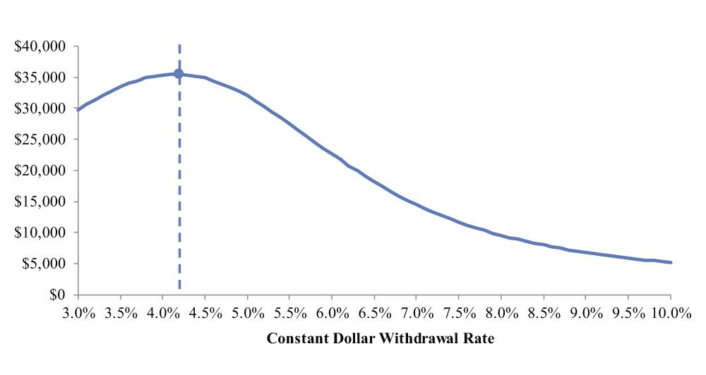
The asset allocation decision should not be made independently from the withdrawal rate decision. In our baseline scenario, we find the optimal withdrawal amount for the rising equity glide path (20% to 70%) is 4.2%. A 4.2% withdrawal increases the certainty equivalence to $35,488 (Figure 2).

Figure 2. Average Certainty Equivalence Assuming
$0 Pension, $1 Million in Savings and a 20% to 70%
Rising Equity Glide Path

 

The 30-year success rate with a 4.2% withdrawal is 70.8%. When combined with mortality assumptions, we find that this pattern would cause about 14.9% of married households retiring at age 65 to completely exhaust savings (with this conservative market return assumption). This represents a balance between the potential for running out of money and the potential for underspending during retirement.

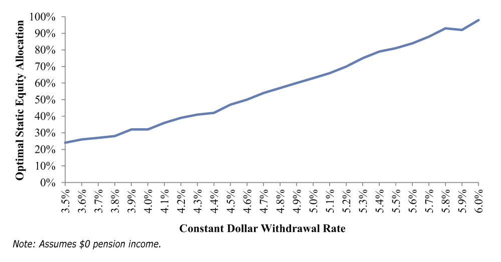
For a household that needs a higher withdrawal rate, it may be optimal to allocate more aggressively to equities. On the one hand, worst-case outcomes will be worse when aggressive withdrawals are coupled with aggressive allocations. On the other hand, a conservative allocation with an aggressive withdrawal has little chance of success. An aggressive allocation gives the best chance on average for an aggressive withdrawal to last.

Figure 3 shows how the optimal static equity allocation increases as the withdrawal rate increases. We look only at the optimal static equity allocation here, with the understanding that a rising equity glide path may help incrementally. This is the first justification for the benefit of rising equity glide paths. A constant dollar withdrawal will become a higher percentage of the remaining portfolio as savings decrease over time. This higher percentage withdrawal suggests a higher equity allocation over time, aligning with a rising equity glide path.

Figure 3. Optimal Static Equity Allocation by
Constant Dollar Withdrawal Rate

Pension Income

We now look at results when pension income is included. Although few working households today will receive a corporate pension, most will receive Social Security and many households nearing retirement have some remnant of a pension. The Survey of Consumer Finances shows that about half of households aged 55 to 64 expect to receive between $30,000 and $50,000 per year in guaranteed retirement income, inclusive of Social Security.

Guaranteed income should have the effect of increasing the optimal withdrawal rate and equity allocation. The logic is straightforward: A household may be willing to take more risk with savings when failure leaves it with some guaranteed income as opposed to none. Exhausting savings and having $0 income must be avoided at all costs, whereas exhausting savings and having $40,000 income is slightly more tolerable. This is one of the central points of Moshe Milevsky and Huaxiong Huang’s paper, “Spending Retirement on Planet Vulcan: The Impact of Longevity Risk Aversion on Optimal Withdrawal Rates” (March/April 2011 Financial Analysts Journal; republished in the September 2011 AAII Journal).

Figure 4. Average Certainty Equivalence
Assuming a 5% Withdrawal Rate, $40,000
Pension and $1 Million in Savings

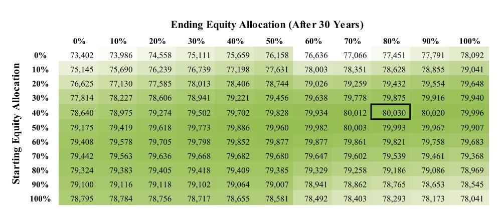
When we include $40,000 of guaranteed income, the optimal withdrawal rate with a static 50%/50% portfolio is 5%. It is higher than the 4.2% withdrawal rate we found earlier because the utility-maximizing household is willing to tolerate increased risk since the downside is not as calamitous. The optimal glide path also increases exposure to equities, starting with an allocation of 40% and increasing to 80% (Figure 4). Again, the household is more willing to tolerate asset risk (price volatility) because of the safety net provided by the guaranteed income. We confirm in our model that the optimal withdrawal rate and equity allocation increase as guaranteed income increases compared to savings (Figure 5).

This is the second reason that rising equity glide paths make sense. With a pattern of declining savings, guaranteed income becomes relatively more important over time. When guaranteed income is the primary component of retirement income, it is optimal to accept more risk with exposure to equities.

We should also point out here that as guaranteed income becomes a more important component of overall retirement income, the improvement from rising equity glide paths shrinks. The certainty equivalence for the optimal glide path is only about 0.1% higher than for the static 50/50 allocation.

Figure 5. Optimal Withdrawal Rate and Static
Equity Allocation by Guaranteed Income Amount

Conclusion

This article provides two mathematical explanations for why rising equity glide paths may improve performance, albeit by a small amount.

First, calibrating an appropriate withdrawal rate is critically important for maximizing utility. The withdrawal rate and equity allocation decisions must be coordinated. A higher withdrawal rate may require a more aggressive equity allocation. Likewise, a higher equity allocation may allow for a higher withdrawal rate. If retirees are spending from principal, as they are in our model, then a constant dollar withdrawal will become a higher percentage of the remaining portfolio. As the withdrawal percentage increases, we have shown that it is optimal for the allocation to equities to increase as well, consistent with the rising equity glide path.

Second, the results from this paper and others show that optimal equity allocations and withdrawals increase as the ratio of guaranteed income to savings increases. Again, this is consistent with the advantages of the rising equity glide path. If retirees are spending from principal, then pension and Social Security income become relatively more important sources of income. The logic follows that it is optimal to increase exposure to equities as savings shrink.

These results highlight two reasons that help explain why rising equity glide paths may be optimal for many households.

Related

Portfolio Strategies

Increasing Retirement Withdrawal Rates Through Asset Allocation

Related

Portfolio Strategies

Reduce Stock Exposure in Retirement, or Gradually Increase It?

Related

Financial Planning

Retirement Spending on Planet Vulcan: Longevity Risk and Withdrawal Rates