Allocating investments through time to satisfy income during retirement is not the same as maximizing wealth at the date of retirement. Some fund managers portray the maximum wealth objective as a proxy that satisfies the retirement income objective, and use ‘glide paths’ to manage portfolio risk. But this approach ignores the risk of income sufficiency, especially for healthy retirees living beyond life expectancy. [Editor’s note: A glide path is the planned change in a portfolio’s allocation over time.]

Portfolio glide paths accommodate investment growth in early working life and transition to lower-risk portfolio settings near retirement. The success of this design hinges on its objective to amass wealth at the date of retirement. But this approach offers little in the way of a solution for the provision of income during retirement. In this article we demonstrate that glide paths can be personalized for individuals to maximize expected retirement income sufficiency under a range of assumptions, including longevity risk.

Target-date retirement funds (TDFs) have become widely popular to mitigate the risk profile of wealth portfolios. These funds initially commit a high allocation to stocks followed by a shift toward less volatile assets as the target retirement date approaches. The result is a glide path that claims to offer the best of both worlds: portfolio growth that can accommodate volatility during the early years followed by the preservation of accumulated wealth near retirement. The glide path is programmed to offer investors assurance that there is no need to keep constant watch over their investment strategy. Indeed, it acts as an antidote to the behavioral inertia manifested by the usual reluctance of investors to change their asset allocation through time.

The vulnerability of such an approach is becoming clear as seasoned target-date fund investors enter retirement. At the date of retirement, the need for reliable income suddenly overrides concerns over arbitrary notions of portfolio value. While glide paths represent the allocation differential between lower risk and higher risk assets over time, they offer nothing toward the capacity of wealth translating into income, which may need to last for the duration of a potentially lengthy retirement.

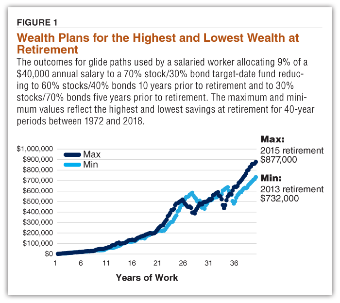
To demonstrate the flaws in arbitrary glide path design, Figure 1 illustrates the wealth paths to the date of retirement for a salaried worker over 40 years of working life, allocating 9% of a $40,000 annual salary to a 70% stock/30% bond target-date fund, reducing to 60% stocks/40% bonds 10 years prior to retirement and to 30% stocks/70% bonds five years prior to retirement. In the past few years, the best outcome was achieved for an individual starting work in 1975 and retiring in 2015. The worst outcome was for a someone starting work in 1973 and retiring in 2013, merely two years earlier. The best outcome would provide 75% of a worker’s final salary over 25 years of retirement, while the worst outcome would provide only 63% of a final salary over the same period. Only two years of working life separate the best and worst outcomes, and yet the difference in retirement wealth is roughly $145,000. This is equivalent to three years’ salary.

So, what happened? The glide path approach has enforced arbitrary asset allocation decisions at discrete, predefined dates. Bad timing in switching allocations has merely crystalized poor portfolio performance at the worst possible time, with the subsequent loss in aggregate wealth being largely irrecoverable. This is a critical failing for workers approaching retirement.

Glide path design is not without value. It attempts to synchronize risk with the risk tolerance of individuals. However, we believe that wealth management using this approach is solving for the wrong objective. The relevant risk should be retirement income uncertainty, not portfolio volatility or total wealth at retirement.

Retirement income planning is extremely sensitive to the objective function specified. It is an asset-liability management plan designed to mitigate mismatches between retirement assets and liabilities enshrined in the demands and commitments governing individual behaviors. For an asset-based objective function, the criteria for performance is ‘time-weighted.’ For an income-based objective function, the criteria for performance is ‘wealth-weighted.’ The asset-based approach envisions risk as the second moment of a portfolio distribution (the standard deviation or, more popularly, volatility); an income-based approach views risk as a complex system characterized by both risk and uncertainty, especially with regard to the longevity of an individual.

Dynamics of Retirement Incomes

A long-ignored challenge in retirement income planning is to better understand the actual spending patterns of retirees. It is generally assumed that retirees desire a constant level of expenditure in real terms through retirement, motivating growth in retirement annuity products in the 1980s and 1990s.

However, observations of actual spending patterns deviate from this assumption dramatically. While spending is stable in the first few years in retirement, significantly lower spending in real terms generally occurs at older ages; for older retirees there is no increase in spending, it merely stops falling.

U.S. data reveals that, in the absence of unexpected medical expenses, the cost in late retirement is no more than that observed in mid-retirement. In other places like the U.K., Australia and Canada, a greater portion of medical costs are borne by the government, so late-retirement spending tends to be even lower. Therefore, retirement income needs are variable and usually decline with age.

Probabilities for Financial Peril Under Different Scenarios

To quantify income sufficiency risk, we need a measure for the risk itself. The notion of financial ‘ruin’ is often overly simplified. Individuals do not usually experience financial ruin at a discrete point in time; rather, they adapt and adjust their consumption relative to savings and expected longevity, and most avoid the discrete realization of ruin as an absorbing state. The depletion of their wealth will tend to be asymptotic and, given the capacity to sell other assets and benefit from state-based forms of social security, individuals are unlikely to become destitute upon exhausting this source of wealth. To appropriately account for measures of income sufficiency, we use financial ‘peril’ in place of ‘ruin’ to reflect the distress associated with income insufficiency.

We demonstrate our approach using a simulation for a ‘model’ worker. Consider an individual facing 40 years of working life until retirement at age 65. Our worker contributes 10% of their annual $40,000 salary to a retirement portfolio. Salary growth is 1% per annum in real terms, and contributions and nominal earnings are taxed at 15%. Upon retirement we assume the worker wishes to withdraw 70% of their final salary as income each year. If wealth is depleted before the end of the 30-year retirement period, then the portfolio reaches an absorbing state of wealth depletion (financial ‘peril’), and no further withdrawals are possible.

Assume that only two assets are available to the investor: 1) stocks, represented by the S&P 500 index and 2) bonds, represented by the Barclays U.S. Investment-Grade Bond index. Correlation between the asset classes is a constant 0.20.

Using a Markov chain Monte Carlo simulation approach (which considers the probabilities of different scenarios), we model the full range of alternative glide path profiles across the individual’s working and retirement life. We use historical risk-return data for U.S. stocks that also accounts for skewness (asymmetric returns) and kurtosis (increased likelihood of extreme returns relative to a normal distribution). To cater to the forward outlook for lower-than-historical-average interest rates, we apply forward projections of returns for U.S. bonds based on the 10-year U.S. Treasury note rate (0.85% per annum) and the option-adjusted spread for U.S. investment-grade bonds (1.65% per annum). While blending historical data with forward data is not generally preferred, this does provide a reasonable forward projection that caters to contemporary risk-return profiles of each asset class. Table 1 provides a summary of the simulation assumptions.

Table 1. Assumed Asset Class Returns for Simulations

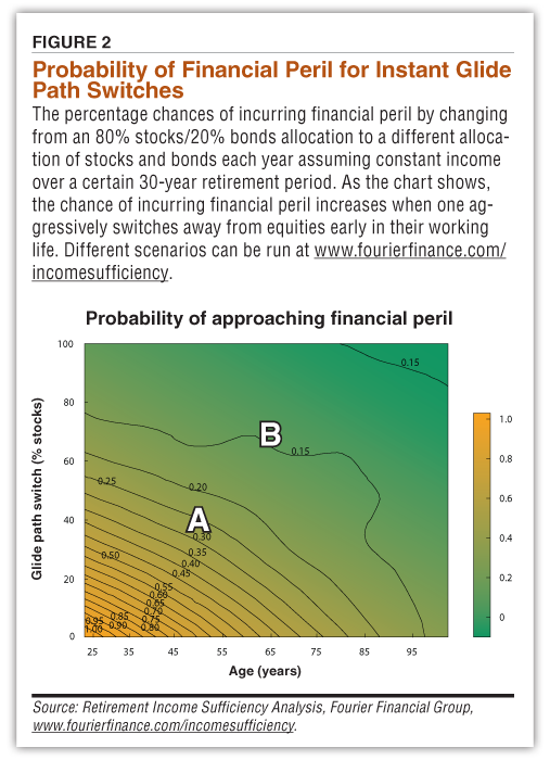
The simulation applies a 10-year linear glide path from an initial allocation of 80% stocks/20% bonds to a new allocation, as represented by the y-axis in Figure 2. The simulation produces a contour plot which illustrates relative zones of peril for a range of glide path switching profiles over a 70-year period (ages 25 to 95). Final allocations with a smaller stock component will therefore exhibit steeper glide paths. As we move along the x-axis, the older the worker gets and the later the glide path switch is made. This profile assumes the retiree withdraws a constant income equivalent to two-thirds of the salary at retirement for 30 years.

The contour plot demonstrates the probabilities of financial peril for each glide path switching profile alternative. Point A indicates a 25% probability of financial peril for a glide path initiated at age 50 that switches from an 80% stock/20% bond portfolio to a 40% stock/60% bond portfolio. Point B indicates that—for the same individual—delaying the glide path until age 65 and then switching to a 70% stock/30% bond mix lowers the chances of peril to less than 15%. Different glide path profiles and commencing ages will alter the probability of financial peril, and the contours describe zones of equivalent peril.

Aggressively switching to conservative allocations prior to retirement has a deleterious effect on retirement income sufficiency. For example, a switch from stocks to a portfolio with greater than 80% bonds early in an individual’s working life results in a high probability of financial peril, in terms of retirement income sufficiency. Portfolio risk is certainly lowered but, then again, so is the potential for a healthy retirement income.

Switching to a 60% stock/40% bond portfolio and maintaining this level throughout both working life and retirement offers a slightly reduced probability of financial peril of roughly 20%. Postponing the switch by 20 years reduces the probability of financial peril to under 20%. However, maintaining a high (80%) allocation to stocks or switching to an even higher allocation results in roughly the same probability of financial peril. In this case, retaining higher allocations to stocks for longer and potentially experiencing higher portfolio volatility would therefore be unnecessary. These baseline assumptions mean that the average worker could accumulate sufficient wealth to avoid financial peril roughly 80% of the time without incurring greater risk than necessary.

The contour depiction fully describes glide path alternatives facing this individual from which to make asset allocation decisions that minimize the risk to retirement income sufficiency. Note that we do not discount the value of glide paths as a risk management tool. Rather, we alter the way in which glide paths are applied and personalized to an individual’s circumstances. Individuals facing different situations based on their age, portfolio contribution rate, required retirement income, salary growth and expected longevity will estimate different contour plots that offer an asset allocation profile specific to them.

To test the sensitivity associated with varying the retirement date, the same simulation can be performed where, 1) the retirement date has been brought forward, or 2) the retirement date has been extended. Automatic glide paths that switch toward conservative assets increase the probability of financial peril by roughly 5% for every year that a worker is forced to enter retirement earlier than expected. In contrast, workers who are able to extend their working lives can either more comfortably switch to conservative assets during their working life without a substantial effect on retirement income sufficiency or maintain their asset allocation and greatly reduce the probability of financial peril. The decrease in probability is roughly 5% for every year a worker is able to extend the date of retirement, but this rate diminishes rapidly as the probability of financial peril becomes almost negligible for those able to retire much later (i.e., beyond the age of 70).

Managing Longevity Risk

Asset allocation choices and sensitivities related to longevity risk can also be tested through this approach. For instance, the chances of a U.S. woman worker living to 98 is roughly equivalent to the chances of her dying before age 70. We can account for longevity when addressing income sufficiency through glide path profile alternatives using the contour profiles. We find that longevity can be managed using a different allocation profile, where switching to less risky assets does not necessarily result in an acute rise in the probability of financial peril. Aggressive asset management for these types of investors would be less critical.

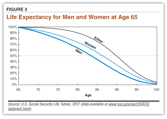
Using mortality tables (U.S. life expectancy for 2017), there is a 12% chance for a single woman to live to 95 and a 6% chance for a single man to do so. For a couple, the chances of at least one member of the couple being alive at age 95 is almost 20% and the chances of one partner surviving to age 100 is almost 5%. Figure 3 illustrates the life expectancy for men and women singly and as a couple. The contour plots for an unusually lengthy retirement show that aggressive allocation to riskier assets is not needed and the optimal outcome would be for an 80% stock/20% bond split to be held constant throughout both working and retirement periods.

Underestimating life expectancy can greatly accelerate the chances of financial peril. For instance, extending longevity by five years for the worker analyzed in Figure 2 results in an increased probability of financial peril by 20%. Extending longevity by 10 years increases the probability by 50%. But sensible asset allocation strategies that avoid simplistic glide path profiles can address longevity risk.

For instance, retaining a 70% stock/30% bond allocation beyond the retirement date will result in the same risk of financial peril as for a 50% stock/50% bond allocation if longevity is extended unexpectedly by five years. An allocation of 90% stocks/10% bonds would achieve the same outcome if longevity were extended unexpectedly by 10 years.

Postponing retirement is an effective antidote to longevity risk. Using the same example, retiring two years later is sufficient to offset an additional five years of longevity without the need to substantially alter asset allocation. Retiring three years later is sufficient to offset over 65% of the risk for an additional 10 years of longevity.

Another issue is that current glide path methods assume the date of retirement is at the choosing of the individual. However, many workers are not lucky enough to choose the date of their retirement; in many cases it is chosen for them. For a fixed retirement date, appropriate asset allocation and greater portfolio contributions are the two most effective possible mechanisms available to investors to mitigate longevity risk. First, avoiding aggressively allocating to conservative assets at any point prior to retirement (especially allocations to bonds of more than 30%) and increasing contributions from salary are very effective strategies. Second, additional salary contributions can directly address the risk, but become less impactful as a worker nears retirement.

Few individuals experience a continuous working life followed by a smooth transition to retirement. Many take career breaks to raise children, others retrain and shift careers. Some individuals will be forced into early retirement while others will choose to retire early given a portfolio wealth threshold. The key advantage of this approach is the ability to map an individual’s glide path as circumstances change, so that suboptimal asset allocation actions can be avoided.

Personalized Glide Paths

Performing these simulations demonstrates that personalizing glide paths can be conducted at any stage in life, especially at discrete instances when circumstances change (e.g., household income alters sharply due to changes in family responsibilities, career change, windfalls through inheritance, etc.). Anticipating significant changes in salary, likely age of retirement, family circumstances, retirement income needs due to illness and so on can and should be used to dynamically update optimal glide path profiles.

Updating glide path strategies upon learning of significant life changes in a reactive way avoids many of the restrictive assumptions of homogeneity among the worker populations. The contour plots can easily reveal differences in the chance of financial peril being affected by early/late retirement, increased longevity, investment returns and volatility and contributions.

We suggest that the optimal way to apply this technique is to use the range of static assumptions as inputs to refresh the glide path for individuals as facts and circumstances change. A free version of the retirement income sufficiency model is available at www.fourierfinance.com/incomesufficiency.

Conclusion

Glide paths are not, in themselves, inefficient. But their arbitrary design under all circumstances for all individuals assumes a level of homogeneity among workers that doesn’t exist in reality.

The use of observed income profiles can be efficiently incorporated into glide path designs to maximize retirement income sufficiency. Whole-of-life contribution and retirement income modeling that minimizes retirement income uncertainty produces glide path profiles that can be personalized for individuals.

Related

Financial Planning

Five Major Considerations for Early Retirement

Related

Financial Planning

Increasing Your Retirement Resources: The Power of Working Longer

Related

Portfolio Strategies

The Mathematics of Retirement Portfolios