One method of judging how aggressive a company’s executives are being with their accounting decisions is to look at accruals.

Accrual accounting recognizes transactions when their economic benefits become probable. Cash accounting, conversely, recognizes transactions when cash exchanges hands.

Put another way, accruals can be described as forecasts of future economic benefits. For example, inventory may be purchased in anticipation of future sales. Under cash accounting, these expenses would be immediately recognized. Accrual accounting, however, allows the expenses to be matched against future sales. As long as the sales actually do materialize and the company receives payment for them, there is nothing wrong with accruals. A problem arises when either future sales do not actually occur, actual revenues are less than anticipated and/or the payment from customers are not received. Such events create a mismatch between income and cash flow leading to write-downs and worst-performing stock prices.

The link between relatively high accruals and lower future stock prices is known as the “accrual anomaly.” It is credited to Richard Sloan, an accounting professor at the University of California–Berkeley. Sloan’s finding is used in several exchange-traded funds focused on quality, including iShares Edge MSCI USA Quality Factor ETF (QUAL) and PowerShares S&P 500 Quality Portfolio ETF (SPHQ). In this article, I explain why accruals can be problematic and how to determine whether a company is being overly aggressive with its use of accrual accounting.

To fully understand the accrual anomaly, it helps to be familiar with the interplay between financial statements. Those unfamiliar with these statements or simply needing a refresher may find it useful to read three past AAII Journal articles in our Financial Statement Analysis series: “Getting to the Bottom Line: How to Read the Income Statement” (May 2024), “Balance Sheet Basics: Demystifying What a Company Owns & Owes” (July 2024) and “Money in, Money out: What the Cash Flow Statement Reveals” (September 2024)

A deep understanding of accounting is not required, however, to simply determine whether a company is being overly aggressive with its use of accruals. A simple equation discussed in John Bajkowski’s April 2017 First Cut: “Stocks With Attractive Accrual Ratios” works well and can be calculated with just a basic calculator and a sheet of paper.

The equation uses cash from operations (found on the cash flow statement), cash from investing (found on the cash flow statement) and net income (found on the income statement) for the recently reported 12-month period (12m) plus total assets (found on the balance sheet) for the most recently reported quarter and the same quarter one year prior [e.g., first quarter of 2017 (Q1) and the first quarter of 2016 (Q5)]. Positive numbers suggest an aggressive reliance on accruals, less persistent earnings and a greater likelihood of a write-down being taken within the next year or two. Negative numbers suggest a higher cash (as opposed to accrual) component of earnings. These latter companies are more likely to have persistent earnings and be less likely to write down the value of their assets in the future.

How Accruals Work

To show how accruals work, I use two new fictional food truck businesses; one operated by Bob and the other operated by Sue.

Bob, having never operated a food truck before, decides a more cautious approach is warranted at first. So, he rents a food truck for just the day at $1,000. He purchases $1,000 worth of food for his first day, too. After finding a good lunch-time spot, Bob sells out of all the food he has prepared, realizing $2,500 in revenues. Bob isn’t yet ready to take credit cards, but is fortunate enough to have all his customers willing to pay in cash.

Bob’s profit for the first day is $500. He spent $2,000 on the truck and food. He realized $2,500 in revenues—all cash transactions. This makes the $500 difference a cash profit. (The math is $2,500 – $2,000 = $500.)

Sue hasn’t operated a food truck before either, but feels good about her chances of succeeding. Rather than rent, she buys a truck for $30,000 in cash. The truck isn’t in the best shape, but Sue has limited amounts of money to work with. Her plan is to get the truck to last 30 days and then use her profits to buy a better truck.

Accrual Ratio Formula

 

Like Bob, Sue spends $1,000 on food and realizes $2,500 in revenues on first day. She isn’t set up to take credit cards on her first day. Rather than miss out on sales, Sue tells the half of her customers who do not have cash on them that they can pay her tomorrow when she hopes to be able to accept credit cards.

Sue’s profits for the first day are $500. Sue earned the same amount of profits as Bob thanks to accrual accounting. A quick walk through the math will explain how this possible. Sue spent $30,000 on the truck, but thinks it will last 30 days. This means the truck will depreciate at a rate of $1,000 per day, making her depreciation expense for her first day $1,000. Sue’s food costs are $1,000. Her total expenses are therefore $2,000—the same as Bob’s. Like Bob, she realized $2,500 in sales. Hence, she earned $500, just like Bob did.

Two things should jump out at you (beyond any assumptions about what it actually costs to operate a food truck). First, Bob was paid in cash by all his customers, while half of Sue’s customers have yet to pay her. There is no guarantee that Sue will be paid by the customers she sold food to on good faith instead of actual payment. Second, Sue makes optimistic assumptions about how her business will fare in the future, while Bob is more pragmatic.

Tying this back to the financial statements (displayed in Table 1), Sue’s balance sheet now lists $1,250 in accounts receivable. This is money owed to her by customers for food they purchased. Accrual accounting allows Sue to record the full value of her Day 1 sales on her income statement as long as she lists outstanding amounts owed to her as receivables in the current assets section of the balance sheet and reasonably expects to be paid. Sue’s cash flow statement, however, reduces cash from operations by $1,250 in recognition of the customers who have yet to pay her.

Table 1. Simplified Financial Statements

 

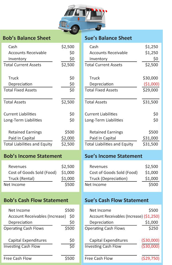
Sue also lists the full value of the truck on the balance sheet of $30,000. Since there was a cash outlay on a fixed asset, she records an outflow of $30,000 in the capital expenditures line of the cash flow statement under cash from investing activities. At the end of Day 1, a depreciation expense of $1,000 is booked to account for the truck’s decline in value due to wear and tear. The depreciation is subtracted from the full value of the truck on the balance sheet to adjust its value. The decline in the asset’s value is a cost and results in the same $1,000 in expenses being recorded on the income statement, reducing profits. No cash was spent by Sue on this expense, however. As such, the depreciation expense is added back to cash from operations on the cash flow statement. (Cash from operations starts with net income and, among other things, adds back non-cash expenses.) All this accounting results in Sue’s free cash flow being –$29,750 ($31,000 in cash outlays less $1,250 in paid transactions.)

Bob’s financial statements are far simpler, as you can also see in Table 1. All his customers paid in cash, so there are no receivables. He rented the truck, so there are no fixed assets and no corresponding depreciation to record. His cash from operations therefore match his net income. He spent $2,000 in outlays and was paid $2,500 by his customers, resulting in total cash flow of $500. Since there are no capital expenditures, he also has $500 in free cash flow.

Sue’s $500 in profits are predicated on the assumptions that the non-paying customers will return and pay for the food and that she’ll get 30 days of use out of her truck. If either assumption proves to be false, Sue will have to write down the value of her receivables, her fixed assets or both. These write-downs will reduce future profits.

The Downside Risk of Accruals

Sue’s risk of not being paid or having her truck not last 30 days highlights a key risk of accrual accounting. In his oft-cited paper, “Do Stock Prices Fully Reflect Information in Accruals and Cash Flows about Future Earnings?” (Accounting Review, July 1996), Sloan wrote, “Current earnings performance is less likely to persist if it is attributable primarily to the accrual component of earnings as opposed to the cash flow component.”

Bob’s earnings are fully attributable to the cash component. He paid for all his expenses in cash, the truck was rented and all his customers paid him at the time of sale. No matter what happens to Bob’s food truck business in the future, there is nothing to cause him to take a future write-down based on his Day 1 operations. Sue, on the other hand, has to hope not only that her non-cash carrying customers show up and pay, but also that she gets more use out of her truck. If she doesn’t get paid by all of her customers or her truck does not last 30 days, she’ll have to take a write-down, which will thereby reduce future earnings. Of course, if the truck can be used beyond its 30-day expected life, earnings will benefit since the truck will be fully depreciated and no charge will be required against revenues.

Extending the conversation to corporations, accruals can play out in a few ways. One involves inventories. If a company stocks up on inventories, its book value will grow (inventories are a current asset), but cash from operations will be reduced (cash was spent to purchase the inventories, though the reduction in cash from operations won’t be recognized until the company pays its suppliers, much like an electric bill does not alter your checking account balance until you pay the utility.) Current earnings won’t be affected since the purchase does not alter sales or profitability if it is in addition to existing inventory being used to fulfill current sales. The company increases its inventory in expectation of a future economic benefit, meaning profitable sales. Actual future earnings will be influenced by whether the inventory is sold above or below its cost.

Let’s use sweaters as an example. A retailer expecting a cold winter buys $50,000 worth of sweaters in September. Assuming the retailer paid for the sweaters before the third quarter was over (and thereby not accruing an accounts payable on the balance sheet for the amount owed), inventory was increased, but profits were unaffected. The third-quarter cash flow statement reflects an outflow of $50,000 to account for the purchase. Winter turns out to be much milder than forecast and hurts demand for sweaters. In February, seeing half of the sweaters still unsold, the retailer decides to mark down the remaining inventory to half of its cost. Though the sweaters are finally sold, a charge of $12,500 is booked against first-quarter profits ($25,000 worth of sweaters sold for $12,500.) This charge reduces first-quarter earnings, decreases book value (the sweaters were sold below their record value), but adds back $12,500 to the operating cash flow. (The initial outlay of $50,000 had previously been recorded. The influx of $12,500 increases cash inflows for the quarter in which payment was received from customers or their credit card companies.)

Note that in this example, earnings for the third quarter would have differed from cash flow. The retailer spent $50,000 on sweaters, which reduced cash flow but not earnings in the third quarter, assuming no factors outside of this example. (There was a cash outlay, but no sales or profits related to the transaction in the same quarter.) This caused earnings to be higher than cash from operating activities. In the first quarter of the following year, earnings were reduced by the write-down, but cash flow was unchanged from this non-cash expense. This fact demonstrates the persistency of cash earnings relative to accrual earnings. Earnings attributable to accruals are less persistent because if management is too optimistic write-downs will eventually need to be taken. These write-downs will reduce future profitability.

Sloan observed that the change in current accruals is primarily attributable to changes in accounts receivables (money owed by customers) and inventories. These two balance sheet items are subjective and require management projections about what is likely occur in the future. While malfeasant steps on the part of companies (e.g., pushing through more inventory to suppliers and distributors than they would be able to sell during normal business operations—a behavior known as “channel stuffing”) can result in less persistent earnings, the reversal of an accrual through a future write-down is often simply caused by a bad projection made by management. These bad forecasts can be influenced by an executive’s desire to use overly optimistic projections to make current earnings look better or by having too rosy an outlook and ignoring or downplaying contrary evidence.

In a 2013 Journal of Accounting and Economics paper (“Accrual Reversals, Earnings and Stock Returns”), Eric Allen, Chad Larson and Richard Sloan differentiated between good and bad accruals. Good accruals are those that correctly anticipate future economic benefits (e.g., customers pay as expected). Accrual estimation errors are accruals whose future benefits are not likely to be realized. Determining which is a good accrual and which is an estimation error can only be done in retrospect, however. In other words, accrual accounting itself is not bad, but high relative levels of accruals should be viewed as a warning about the potential for lower earnings in the future.

Accruals’ Effect on Stock Returns

In his 1996 paper, Sloan found that a portfolio constructed of stocks with the lowest 10% of accruals realized a size-adjusted return of 4.9% for the first year after formation. A portfolio of stocks with the highest 10% of accruals lost 5.5% during the first year after formation. This resulted in a hedged portfolio composed of buying the lowest accrual stocks and short-selling the highest accrual stocks gaining 10.4% during the year following portfolio formation. The analysis period used firm years for the period of 1962 to 1991.

The hedged portfolio is important because it refers to how anomalies are identified and tracked. An anomaly is said to exist, in part, if a positive return can be realized by going long (buying) stocks at one end of the spectrum and shorting (short selling) stocks at the other end of the spectrum.

The reason for bringing the point up is because more recent studies have suggested that it has become much more difficult to profit from the accrual anomaly. Two key reasons are given. First, it’s harder to arbitrage based on the anomaly. The strongest profits now exist in stocks with low liquidity; such stocks have high trading costs for institutional traders. Secondly, sell-side brokerage analysts appear to be more aware of the impact that accruals have on earnings and are factoring in accruals into their analysis.

Note that neither of these developments implies high accrual stocks are no longer risky. In fact, a 2015 paper written by authors from the University of Chicago and the National Bureau of Economic Research (“Accruals, Cash Flows, and Operating Profitability in the Cross Section of Stock Returns,” Ray Ball et. al, SSRN) bluntly stated, “Firms with high accruals today earn lower future returns because they are less profitable on a cash basis.” Calculating returns from 1963 through 2014, Ball and his co-authors found that a value-weighted portfolio composed of stocks with the lowest 10% of accruals realized a 0.35% monthly excess return advantage over a value-weighted portfolio composed of stocks with the highest 10% of accruals. (The study used average monthly returns in excess of one-month Treasury bill rates.)

A May 2017 study critical of most anomalies, (“Replicating Anomalies,” Kewei Hou et. al, National Bureau of Economic Research), observed a –0.27% per month high-minus-low average return for operating accruals. In other words, high-accrual companies underperformed low-accrual companies by 0.27% per month. The Hou study excluded micro-cap stocks.

The timing of when high accruals will hurt shareholders appears to be within two years. Though this may seem like a long enough period to get out, two caveats should be noted. First, the predictable returns for low-accrual companies are concentrated around subsequent earnings announcements. Put another way, the persistency of their earnings is recognized when companies report their quarterly results. High-accrual companies, conversely, are more likely to preannounce. Since most companies do not preannounce earnings on a routine basis, such announcements are unexpected. Secondly, the studies use portfolio formations from when the high accruals are first identified, which may be three or more quarters prior to you realizing it.

Conclusion

From the standpoint of an individual investor’s portfolio, accruals work best as a measurement of accounting aggressiveness. High levels of accruals should serve as a warning sign that a company may be at risk of a forthcoming write-down, whereas low accruals should reduce worries about such an event occurring in the near term.

Individual investors may find that accrual ratios work best as an added criterion to a stock screen or a list of criteria to evaluate. For example, accruals serve as one component of Joseph Piotroski’s F-Score—a model for assessing the underlying fundamental quality of a company. Various exchange-traded funds (ETFs) combine accruals with measures such as earnings variability to assess quality. An alternative is to simply use accruals as a way to weed out potentially risky stocks. An investor concerned about aggressive accounting practices could simply avoid any stock with a positive accrual ratio.