


Related

Portfolio Strategies
Increasing the withdrawal rate led to bigger distributions, but lower ending wealth. Altering the investing period also has an impact.

Charles Rotblut leads a class in AAII's new Essential Investing Video Course. Go to https://www.aaii.com/ves for more information and to subscribe.
Article Highlights:
This year’s rebalancing update includes a few changes.
First, I’ve adjusted the retirement withdrawals to reflect a higher inflation-adjusted withdrawal rate of 4.5%. This change was made based on updated research by William Bengen as discussed in the January 2018 AAII Journal (“Insights on Using the 4% Withdrawal Rule From Its Creator”).
Secondly, I am introducing rolling period analysis. Since the models now contain 30 years of actual return data—inclusive of the impact of mutual fund fees—I am able to start looking at rolling 25-year-period performance. The sample size of rolling periods is small, but it does offer some insights on how the returns differ depending on the starting period used.
Finally, to shed some light on the relative performance of our moderate portfolio allocation, I have begun tracking the performances of a more aggressive portfolio invested completely in the S&P 500 index and a more conservative portfolio following a traditional 60% large-cap stock/40% bond allocation.
One change that didn’t occur was the portfolios themselves. Even with last year’s big rise in the major stock market indexes, neither the rebalanced non-withdrawal nor the rebalanced withdrawal portfolios required any adjustments. The allocations for both stayed within their respective target ranges for a fourth consecutive year.
Before getting into details, I want to provide some background as a refresher for those who have been following these annual updates and an introduction for those who are new to them.
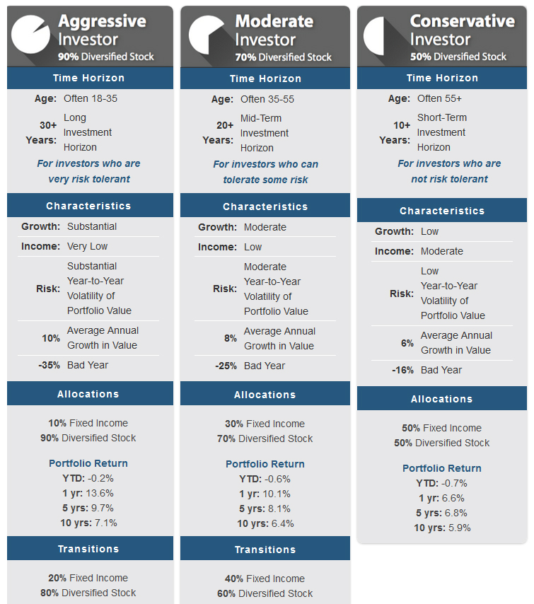
Since 2011, I’ve been conducting an ongoing analysis of hypothetical portfolios based on AAII’s moderate asset allocation model. This model calls for allocating 70% to a diversified collection of stocks and 30% to bonds. For the stock portion, the target allocation I’ve used is 20% in large-cap stocks, 20% in mid-cap stocks, 10% in small-cap stocks and 20% in international developed country and emerging market stocks. See Figure 1 for an illustration of the investor characteristics for the moderate model, as well as the characteristics for two other asset allocation models—aggressive and conservative.
The hypothetical portfolios are either non-withdrawal or withdrawal. No withdrawals are taken out of the first one (the “non-withdrawal” portfolio). The second, the “withdrawal” portfolio, assumes a retiree makes annual withdrawals based on an inflation-adjusted 4.5% amount. (The withdrawal rate is discussed in more detail later in this article.)
Non-rebalanced portfolios established an allocation at the beginning with no further changes being made. Rather, their allocations evolve based on the weighted performance of each fund held. The rebalanced portfolios are periodically adjusted back to their targeted allocations whenever the weighting of any single fund is more than five percentage points above or below its target. The 5% band is based on a Vanguard study (“Best Practices for Portfolio Rebalancing,” AAII Journal, May 2011.)
The hypothetical portfolios use Vanguard funds to replicate the returns an investor could have realized after fund fees are factored in. A start date of 1988 was used because it was the first full year that return data was available for some of the funds used in the models. The models are updated annually using end-of-year return data. Online spreadsheets with the full data and a thorough explanation of the calculations are linked in the online version of this article.
Last year was a very good year to have a significant allocation to equity funds. Both the Vanguard 500 Index fund  (VFINX) and the Vanguard Mid-Cap Index fund (VIMSX) had their best year since 2013. International stocks had an even better year, with the Vanguard Total International Stock Index fund (VGTSX) rising by 27.4%, the biggest increase since 2009.
The big returns caused strategies designed to reduce relative volatility, such as rebalancing, to lag in terms of comparative performance. The non-rebalanced non-withdrawal portfolio realized 19.9% total return in 2017 versus a 16.4% total return for the rebalanced non-withdrawal portfolio.
As shown in Table 1, the difference is attributable to the non-rebalanced non-withdrawal portfolio’s 88.7% allocation to equities. This is 14.0 percentage points higher than the equity allocation of the rebalanced non-withdrawal portfolio. By not rebalancing, the allocation to stocks has been allowed to rise over time. Consider the effect that the current bull market has had. Since the end of 2008, the non-rebalanced portfolio’s equity allocation has increased by a cumulative 13.5 percentage points.
Table 1. Performance of the Three Strategies
| The data below shows how rebalancing compares to not rebalancing for portfolios with the same starting allocation. The Panic and Sell scenarios assume an investor temporarily switches to an all-bond allocation for one year whenever the S&P 500 index incurs a calendar-year drop of greater than 20%. The 60/40 and the S&P 500 Only portfolios are included to provide comparative benchmarks. The 60/40 portfolio was rebalanced annually to an allocation of 60% large-cap stocks and 40% bonds. | |||||
| Portfolio Strategy | Rebalance at 5% Thresholds | No Rebalancing |
Panic and Sell When S&P 500 Falls > 20% |
60/40 Allocation | S&P 500 Only |
|---|---|---|---|---|---|
| Non-Withdrawal Portfolio Results (1988–2017) | |||||
| Ending Portfolio Value | $1,450,613 | $1,572,511 | $961,937 | $1,388,324 | $2,034,202 |
| Total Return | 1,350.6% | 1,472.5% | 861.9% | 1,288.3% | 1,934.2% |
| Standard Deviation | 11.9% | 13.6% | 11.9% | 10.8% | 17.5% |
| Annualized Return | 9.3% | 9.6% | 7.8% | 9.2% | 10.6% |
| Largest Drawdown | -$204,880 | -$253,424 | -$183,385 | -$141,084 | -$337,023 |
| Largest Annual Loss | -26.9% | -32.8% | -30.0% | -20.2% | -37.0% |
| Ending Equity Allocation | 74.7% | 88.7% | 81.5% | 63.8% | 100.0% |
| Ending Fixed-Income Allocation | 25.3% | 11.3% | 18.5% | 36.2% | 0.0% |
| Withdrawal Portfolio Results (1988–2017) | |||||
| Ending Portfolio Value | $600,576 | $700,980 | $365,165 | $605,956 | $1,019,144 |
| Total Return | 500.6% | 601.0% | 265.2% | 506.0% | 919.1% |
| Standard Deviation | 11.6% | 13.2% | 11.6% | 10.4% | 16.9% |
| Annualized Return | 6.2% | 6.7% | 4.4% | 6.2% | 8.0% |
| Largest Drawdown | -$115,009 | -$142,953 | -$107,723 | -$85,902 | -$210,099 |
| Largest Annual Loss | -28.4% | -34.2% | -31.7% | -22.0% | -38.1% |
| Total Withdrawals | $240,032 | $240,032 | $240,032 | $234,910 | $242,307 |
| Ending Equity Allocation | 73.9% | 90.1% | 80.4% | 63.9% | 100.0% |
| Ending Fixed-Income Allocation | 26.1% | 9.9% | 19.6% | 36.1% | 0.0% |
The bigger the equity allocation is, the larger a portfolio’s downside risk will be during the next bear market. This is the trade-off investors must consider when deciding whether to take steps to manage volatility. Long-term wealth is increased by taking on more equity risk, but shorter-term losses are increased—especially during bear markets. Keeping equity exposure within certain boundaries reduces the magnitude of losses at the expense of sacrificing potentially higher long-term returns. Thus, investors must choose between seeking the highest reasonable long-term returns in hopes of achieving greater wealth or taking measures to lower or control risk to reduce the losses caused by corrections and bear markets.
Reducing risk is only one consideration when it comes to rebalancing. Another is the frequency at which the portfolio is rebalanced. Rebalancing too frequently will incur greater transaction costs if commissions and trading costs are a factor. A rebalanced portfolio will also potentially incur a greater return penalty by prompting the investor to reduce exposure to an asset class with good short-term performance.
A systematic approach based on boundaries for each asset class can reduce such costs. The portfolios used in my model only trigger a rebalancing alert if allocation for one of the major asset classes is above or below the target by five percentage points or more. This is based on the aforementioned Vanguard study. The study found that periodic annual or semiannual rebalancing works well with 5% to 10% threshold bands.
These bands have so far proven to be wide enough to limit the number of transactions over time. As previously stated, no rebalancing was required at the end of last year for either the non-withdrawal or the withdrawal portfolios. This marks the fourth consecutive year that neither portfolio has needed to be rebalanced.
The end of this year (2018) could be different. In the non-withdrawal rebalanced portfolio, the fixed-income allocation totaled just 25.3%. Should this allocation fall below 25.0%, the entire portfolio would be rebalanced in order to bring the fixed-income allocation back up to 30%. Whether such an adjustment is actually needed will depend on the performance of the equity funds relative to the bond funds. None of the equity funds is near the top of their allocation ranges, nor do any of them have to be. Simply having an excessive allocation to equities relative to bonds (or vice versa)—and their respective targeted ranges—is enough to trigger rebalancing.
(The withdrawal rebalanced portfolio ended 2017 with more wiggle room. Its bond allocation was 26.1%. The difference in allocation weightings is due to the annual withdrawals taken from this portfolio.)
You can, of course, alter the boundaries for when rebalancing would be required. Those wanting to rebalance less often should use wider ranges. Those more concerned with controlling risk should use tighter ranges. An alternative is to simply rebalance based on time periods. For instance, an investor following the classic 60% large-cap stock/40% bond allocation model would rebalance every year. Rebalancing annually could result in smaller—though more regular—capital gains being realized. Some money managers may rebalance more frequently, such as every quarter. (If you own a multi-asset fund, read the prospectus to find out how frequently the manager rebalances.) Each robo-adviser may have its own strategies for determining how frequently to rebalance.
Capital gains recognized in taxable accounts will lead to a larger tax bill if there are no offsetting losses or other deductions realized to offset them. To the extent possible, use tax-sheltered accounts to rebalance and avoid incurring capital gains taxes. Depending on the nature of your finances, rebalancing in a taxable account may be unavoidable. Such taxes are a cost incurred by rebalancing. In these situations, you will have to weigh the benefits of reducing risk versus incurring taxes. Using wider target allocation boundaries before a rebalancing alert is triggered will reduce the frequency at which taxable transactions occur but could potentially lead to greater periodic capital gains. In investing, there is rarely a free lunch.
As previously stated, I switched to using a 4.5% withdrawal rate in the withdrawal portfolios. The change comes from retired financial planner William Bengen, who created the widely followed 4% withdrawal rule. Bengen found that the higher rate could be used with a diversified portfolio.
For a portfolio with a starting value of $100,000, using a 4.5% inflation-adjusted withdrawal rate would have resulted in $240,032 being withdrawn over the past 30 years. Using a 4% portfolio withdrawal rate instead would have resulted in $213,362 being withdrawn. From an ending-wealth standpoint, the withdrawal rebalanced portfolio was worth $600,576 after the 2017 withdrawal was taken based on the 4.5% withdrawal rate. The same portfolio was worth $695,881 when a 4% withdrawal rate was used.
The difference in cumulative withdrawals does not equal the difference in ending wealth because of the frequency with which the withdrawals were taken. Every time a withdrawal is taken, there is less money in the portfolio to benefit from positive investment returns (or be hurt by negative returns). The annual withdrawals have the effect of gradually reducing how much money is left in the portfolio to grow. At the same time, the 4.5% withdrawal rate leads to increasingly larger dollar amounts being distributed than the 4% withdrawal rate because the starting value is larger. Every inflation adjustment is based on a starting value of $5,181 for the 4.5% withdrawal portfolio and a starting value of $4,605 for the 4% portfolio. (Each portfolio started with $100,000 that appreciated to $115,129 at the end of its first year in 1988.)
The performance of any portfolio is influenced by the time period measured. Both the returns realized and the sequence in which those returns occur will affect how good or bad a portfolio’s performance is. While the sequence of returns doesn’t matter if no changes are made over a specific period (you would have the same ending wealth regardless of whether the good returns occur earlier or later), most investors make at least some changes to their portfolios by adjusting allocations, buying and selling certain securities and funds, contributing additional savings, withdrawing from the account or some combination of these.
Even changing the measurement period by one year can have a very large effect. Look at the returns on Tables 2 and 3. The data shown is for both the non-withdrawal and withdrawal portfolios. The same funds and rebalancing strategies are used, only the starting and ending dates differ. Rather than spanning the full 30-year period of 1988 through 2017, six rolling 25-year periods are used. Each portfolio starts one year later and ends one year later. The sample size of periods analyzed is small because some of the funds used in the analysis do not have full-year data prior to 1988. In future years, I will add to this analysis.
Table 2. Non-Withdrawal Portfolios: 25-Year Rolling Period Returns
| Time Period | Ending Portfolio Value ($) | Total Return (%) | Annualized Return (%) | Standard Deviation (%) |
|---|---|---|---|---|
| Rebalance at 5% Thresholds | ||||
| 1993–2017 | 799,407 | 699.4 | 8.7 | 11.8 |
| 1992–2016 | 646,517 | 546.5 | 7.8 | 12.0 |
| 1991–2015 | 1,026,551 | 926.6 | 9.8 | 13.4 |
| 1990–2014 | 825,093 | 725.1 | 8.8 | 12.4 |
| 1989–2013 | 956,712 | 856.7 | 9.5 | 12.7 |
| 1988–2012 | 907,694 | 807.7 | 9.2 | 12.7 |
| No Rebalancing | ||||
| 1993–2017 | 825,086 | 725.1 | 8.8 | 13.3 |
| 1992–2016 | 756,723 | 656.7 | 8.4 | 13.3 |
| 1991–2015 | 904,109 | 804.1 | 9.2 | 14.0 |
| 1990–2014 | 838,645 | 738.6 | 8.9 | 13.6 |
| 1989–2013 | 949,817 | 849.8 | 9.4 | 14.2 |
| 1988–2012 | 882,268 | 782.3 | 9.1 | 14.1 |
Even with the limited amount of data, a few insights can be drawn.
The first is that a difference of just one year can have a significant impact on the returns that an investor realizes. For example, look at the non-withdrawal portfolios in Table 2. An investor who started in 1988 and ended in 2012, would have far less wealth than an investor whose investing period ran from 1989 through 2013 but used the same exact investment strategy.
What changed? The good year of 1988 was replaced with the great year of 2013. The Vanguard 500 fund gained 16.2% in 1988 and soared 32.2% in 2013. The latter portfolio also had five years to rebound from the 2008 financial crisis instead of four. Finally, the big returns of 2013 occurred at the end of the 1989 to 2013 investing period, when the portfolio’s balance was larger.
These differences highlight how luck plays a role in terms of timing. A period of favorable returns will lead to far greater wealth than a period of bad or below-average returns. A long-term investor has no ability to predict what returns will be over their time horizon.
Second, the relative performance of rebalancing—or any other portfolio strategy—depends on the time period measured. For the non-withdrawal portfolios (Table 2), not rebalancing led to higher returns in three instances, while rebalancing led to higher returns in two instances. For the withdrawal portfolios (Table 3), not rebalancing also had a three-to-two edge. Though the sample size is small, the fact that one strategy does not always outperform the other shows the inherent uncertainty taken when selecting an allocation strategy. Investors always take a risk when choosing an allocation strategy since the outcome is unknowable in advance. It is simply part of the risk that comes with investing. We know that the long-term odds do tend to play out over time.
Table 3. 4.5% Withdrawal Portfolios: 25-Year Rolling Period Returns
| Time Period | Ending Portfolio Value ($) | Total Return (%) | Annualized Return (%) | Standard Deviation (%) | Total Withdrawals ($) |
|---|---|---|---|---|---|
| Rebalance at 5% Thresholds | |||||
| 1993–2017 | 250,950 | 151.0 | 3.7 | 11.7 | 175,900 |
| 1992–2016 | 265,074 | 165.1 | 4.0 | 11.4 | 161,096 |
| 1991–2015 | 350,846 | 250.8 | 5.1 | 11.8 | 192,419 |
| 1990–2014 | 402,723 | 302.7 | 5.7 | 12.2 | 153,096 |
| 1989–2013 | 517,747 | 417.7 | 6.8 | 13.7 | 197,324 |
| 1988–2012 | 458,800 | 358.8 | 6.3 | 12.3 | 188,685 |
| No Rebalancing | |||||
| 1993–2017 | 343,321 | 243.3 | 5.1 | 13.0 | 175,900 |
| 1992–2016 | 266,634 | 166.6 | 4.0 | 12.2 | 161,096 |
| 1991–2015 | 363,853 | 263.9 | 5.3 | 13.4 | 192,419 |
| 1990–2014 | 412,989 | 313.0 | 5.8 | 13.1 | 153,096 |
| 1989–2013 | 397,529 | 297.5 | 5.7 | 13.7 | 197,324 |
| 1988–2012 | 415,928 | 315.9 | 5.9 | 13.7 | 188,685 |
Third, the cumulative number of withdrawals taken depends on when the time period started. An investor whose retirement span ran from 1989 through 2013 would have withdrawn $197,324 cumulatively. The cumulative withdrawals for an investor whose retirement span ran one year later, 1990 through 2014, would have withdrawn just $153,096. The difference is because 1990 was a down year for stocks. The first withdrawal was calculated from a year-end balance of $95,266. Since all future withdrawals are inflation-adjusted based on the first year’s withdrawal, a lower starting withdrawal amount will reduce the cumulative amount of money distributed throughout the remainder of retirement. The reverse is also true: A higher starting withdrawal amount will increase the absolute size of all distributions following it.
Retirees can, of course, adjust their withdrawals if they find their portfolio performance to be better or worse than expected.
To provide some context about the performance of our moderate allocation and the effect of rebalancing, this year I have added two additional approaches as benchmarks. They are portfolios allocated solely to the S&P 500 and portfolios following the traditional 60/40 approach. The S&P 500 portfolio is allocated solely to the Vanguard 500 Index fund (VFINX). The 60/40 approach allocates 60% to the Vanguard 500 Index fund and 40% to the Vanguard Total Bond Market Index fund (VBMFX). The 60/40 non-withdrawal and withdrawal portfolios are rebalanced annually.
The all S&P 500 approach realized the highest returns over the 30-year period of 1988 to 2017. It was also the most volatile. These findings aren’t surprising since the approach is completely allocated to stocks with no bond holdings to buffer the year-by-year fluctuations.
The 60/40 allocation underperformed the rebalanced moderate allocation (70% stock/30% bond) portfolio when no withdrawals were taken. When withdrawals were taken, the ending wealth was similar ($605,956 for the 60/40 versus $600,576 for the moderate allocation). Cumulative withdrawals were slightly higher for the moderate allocation ($240,032) than for the 60/40 allocation ($234,910) because of the higher first-year returns for the former approach.
The results of the all S&P 500 and the 60/40 portfolio are included in Table 1 for comparative purposes. The spreadsheets in the box below show the year-by-year results for all of the approaches. The spreadsheets also contain the year-by-year returns for the funds used and the annual inflation data for those who want to consider other allocation mixes. The spreadsheets include models starting in 1988, 2000 and 2007. The latter two show what happened to portfolios that started just prior to the bursting of the late 1990s dot-com bubble and the start of the 2007–2009 financial crisis.
Also included in the spreadsheets are models demonstrating the long-lasting negative impact of panicking—meaning getting out of stocks following a bad year for the market. The lesson from these models is perhaps the most important: The optimal allocation strategy is the one you personally can stick to no matter what the market is doing.
Complete Data for All Portfolios and Variations
Download the Excel spreadsheets by clicking on each link:
2018 - Rebalancing - 2000 to Present
Portfolio Strategies

Portfolio Strategies
Portfolio Strategies

Chris C from CA posted over 8 years ago:
Bill K from TX posted over 8 years ago:
James Kvitkovich from PA posted over 8 years ago:
You need to log in as a registered AAII user before commenting.
Log InCreate an account